Turn an exploration into one honest page: the question, the data, what was checked, three to five findings each with one number and one picture, the limits, and the next step. Count how much was looked at, and make every number rebuild from the raw table.
Write a one-page report with its six parts: question, data and source, what was checked, findings, limits and next step.
Count the comparisons an exploration made and use a noise simulation to judge which correlations stand out from chance.
Word a finding as an association with its number, its sample size and its limits, never as a cause.
Build the table of findings with one function, so that one script reruns the whole analysis from the raw table.
In review. The maths and code on this page are checked by automated tests on every change, but an independent reader has not signed it off yet. Spot a mistake or a confusing step? Tell us.
The question
You have looked at eleven columns one by one, computed 70 correlations and drawn half a dozen scatter plots. Your reader will look at one page. What goes on it, and what must it admit about everything that did not?
From the last lesson
1. Which measurement correlates most with the score, and how strongly?
Show answer
Body mass index, \({r = 0.59}\), with s5 close behind at 0.57 (and ahead under Spearman’s rank correlation, 0.59 against 0.56).
2. Why do s1 and s2 correlate at 0.90?
Show answer
s2 (LDL) is, for 438 of 442 patients, s1 − s3 − e^s5 / 5: the Friedewald formula. It was computed from total cholesterol, so it moves with it.
Intuition
An exploration produces far more than anyone will read. The report is the last step of the workflow: it keeps the few things that answer the question, says how they were found, and states plainly what the data cannot tell.
S01.8.4-F1
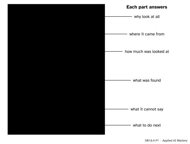
The one-page report. Six parts, each answering one question a reader will ask. The findings are few, and each carries one number and one picture.
Two rules shape the page. Every finding is one number and one picture: the number says how big, the picture shows the shape behind it, as Anscombe’s quartet demanded (S01.5.3). And the page is as honest about the looking as about the results: it says how many comparisons were made before the ones shown, because a pattern picked from many is weaker than one that was sought.
Build it up
The six parts, written for the diabetes table.
1. Question. Restate the question of S01.8.1 in one sentence: which baseline measurements go together with a larger progression score a year later, how strongly, and for which patients.
2. Data and source. 442 patients with diabetes, ten baseline measurements and a score one year later, from the study analysed by Efron, Hastie, Johnstone and Tibshirani (2004), loaded with scikit-learn’s load_diabetes(scaled=False).
3. What was checked. The audit of S01.8.2: no missing values, no duplicated rows, sex a code with no key, s4 a rounded ratio of s1 and s3. Then the count of looks: 11 one-column summaries, 55 correlations among the 11 columns, 15 correlations inside subgroups, 5 scatter plots.
4. Findings, three to five.
The score leans right: median 140.5, mean 152.1. (Picture: the histogram of S01.8.3.)
Body mass index goes most closely with the score: \({r = 0.59}\). (Picture: its scatter plot.)
That link holds in every sex and age group: \(r\) from 0.53 to 0.65. (Picture: the dot chart.)
s5 is close behind at \({r = 0.57}\), and first by rank correlation (0.59).
s2 is computed from s1, s3 and s5 by the Friedewald formula: 438 of 442 match.
5. Limits. Three kinds, always. Who: the patients’ selection is not documented, everyone has diabetes, everyone was scored again a year later, and the table may be what is left after incomplete rows were removed. How measured: units are not stated, s5 is “possibly” a log, the score’s scale is not defined, the sex code has no key. What kind of claim: the data are observational. Nobody was assigned a body mass index, so no finding is a cause (S01.7.3).
6. Next step. Predict the score from the ten measurements and check how well it generalises (ML01.10); put an uncertainty on each correlation (S02); and, for a causal question, a design or a causal graph (S06).
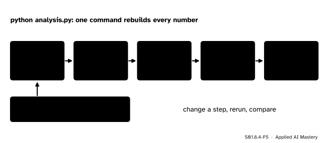
Make it rerun. The page is the output of one script that starts from the raw table, with every random seed fixed (P02.9.4).
S01.8.4-F5
The analysis as one script. Only the raw file and the seed are fixed by hand; every number on the page is rebuilt each time it runs.
A number typed into a report by hand can go stale the moment a cleaning step changes. A number printed by the script cannot.
The formal statement
Counting the looks. With \(k\) columns, each column can be paired with the \({k - 1}\) others. That counts every pair twice, once from each end, so the number of pairs is
\[
\binom{k}{2} = \frac{k(k-1)}{2} .
\]
For \({k = 11}\) that is \({11 \times 10 / 2 = 55}\) (M01.8). Add the 15 subgroup correlations of S01.8.3 and the exploration made 70 correlations.
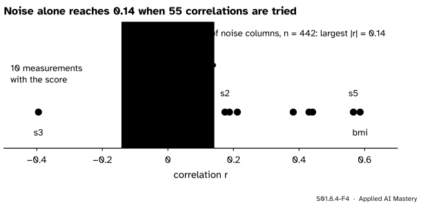
What chance alone can produce. To see how large a correlation can be with nothing behind it, make a table with the same shape and no relationships at all: 442 rows and 11 columns of independent random numbers, drawn with numpy.random.default_rng(0). Compute its 55 correlations.
S01.8.4-F4
Fifty-five correlations among pure noise (grey) and the ten real correlations with the score (blue). Noise reaches 0.14; sex sits well inside that band, the leaders far outside it.
None of the noise correlations is zero. The largest in size is 0.14. Repeating the experiment on 1,000 noise tables, the largest of the 55 is typically 0.12, is below 0.16 in 95 percent of the tables, and never exceeds 0.22. That gives a working rule for an exploration, not a test (tests are S02):
NoteA correlation that chance could have made
When \(m\) correlations were looked at, a correlation no larger than the largest that \(m\) correlations of pure noise reach, on a table of the same size, is not reported as a finding.
By that rule, sex (0.04) is not a finding. s2 (0.17), age (0.19) and s1 (0.21) sit at the edge of what noise reaches, so the report calls them weak. Body mass index, s5, blood pressure, s4, s6 and s3, all above 0.38 in size, are far beyond anything noise produced. Gelman and Loken add a subtler point: even one analysis has many hidden forks (which rows to drop, which groups to form), so the count is a floor, not a ceiling.
Worked example
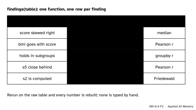
Build the table of findings with one function. Each row comes from a summary written from scratch in this course: the median and mean (S01.3), Pearson’s \(r\) (S01.5.2), the subgroup check (S01.8.3) and the Friedewald check.
S01.8.4-F2
The findings table as the function returns it. The middle column is the only place the report’s numbers come from.
Trace one row by hand, the third. The function splits the 442 patients into the two sex codes and the three age bands, computes \(r\) for body mass index and the score in each of the five groups, and keeps the smallest and the largest: 0.53 (sex coded 1) and 0.65 (sex coded 2). The row reads “holds in subgroups, r = 0.53 to 0.65”. The age bands, at 0.55, 0.61 and 0.54, fall in between.
Now the wording of that finding, built from its parts: who (patients with a higher body mass index at the first visit), what (tended to have a higher score a year later), how much (\({r = 0.59}\), \({n = 442}\)), how sure of its reach (0.53 to 0.65 in five subgroups), how much was looked at (one of 70 correlations) and what it is not (observational, so not a cause).
Code
The findings table, from scratch.
import numpy as npimport pandas as pdfrom sklearn.datasets import load_diabetesSEED =0table = load_diabetes(as_frame=True, scaled=False).framedef corr(a, b): a, b = np.asarray(a, dtype=float), np.asarray(b, dtype=float) da, db = a - a.mean(), b - b.mean()returnfloat((da * db).sum() / np.sqrt((da **2).sum() * (db **2).sum()))def findings(t): bands = pd.cut(t["age"], [0, 39, 59, 120]) groups = [g for _, g in t.groupby("sex")] + [g for _, g in t.groupby(bands, observed=True)] inside = [corr(g["bmi"], g["target"]) for g in groups] rebuilt = t["s1"] - t["s3"] - np.exp(t["s5"]) /5 rows = [ ("score skewed right", f"median {np.median(t.target):.1f}, mean {t.target.mean():.1f}"), ("bmi goes with score", f"r = {corr(t.bmi, t.target):.2f}"), ("holds in subgroups", f"r = {min(inside):.2f} to {max(inside):.2f}"), ("s5 close behind", f"r = {corr(t.s5, t.target):.2f}"), ("s2 is computed", f"{int((abs(rebuilt - t.s2) <0.01).sum())} of {len(t)} match"), ]return pd.DataFrame(rows, columns=["finding", "one number"])report = findings(table)print(report.to_string(index=False))
            finding               one number
 score skewed right median 140.5, mean 152.1
bmi goes with score                 r = 0.59
 holds in subgroups         r = 0.53 to 0.65
    s5 close behind                 r = 0.57
     s2 is computed         438 of 442 match
The count of looks and the noise simulation, with its seed fixed.
DataFrame.agg takes a list of summaries and returns them as a table; corrwith correlates every column with one other. Put the cells of this lesson into one file with SEED at the top, and the report rebuilds itself.
Explore
This module’s interactive, the audit trail, lives in lesson S01.8.2. Before writing a report, fix every fault it finds and note how far each fix moved the numbers: that list is the cleaning log your report’s third part refers to.
Pitfalls
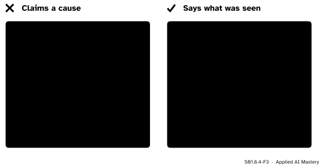
S01.8.4-F3
Wrong beside right. The same finding, written as a cause and written as what was observed, with its number, its sample, its reach and the count of looks.
“Body mass index drives progression.”
Nothing in an observational table can show that. Patients with a high body mass index may differ in diet, age, treatment or the type of their diabetes, and any of these could move the score (S01.7.3). Write “goes with” or “tended to”, give the number, and leave causes to a design that assigns the treatment (S05) or a causal analysis (S06).
“I will only show the plot that worked.”
Showing the strongest of 70 correlations without saying there were 70 makes it look stronger than it is: noise alone reaches 0.14 in 55 tries. Report the count of looks, and keep the dull results in an appendix.
“I will fix that number in the report by hand.”
Then the report and the analysis disagree, and the next rerun overwrites the fix or keeps the error. Change the script, rerun it, and let the page be rebuilt. Machine-learning results that cannot be rerun from the raw data cannot be checked either (ML01.10).
Check yourself
Recall
1. Name the six parts of the one-page report.
Show answer
Question; data and source; what was checked; findings; limits; next step.
2. What does every finding carry?
Show answer
One number (how big) and one picture (the shape behind it), plus the sample size and its limits.
3. How many correlations are there among 11 columns, and why?
Show answer
\({11 \times 10 / 2 = 55}\): each column pairs with the other 10, and that counts every pair twice.
4. What are the three kinds of limit a report states?
Show answer
Who is in the data (selection), how things were measured (units, codes, derived columns), and what kind of claim is possible (association, not cause, for observational data).
5. Why should every number in the report come out of the script?
Show answer
So that the whole analysis reruns from the raw table with fixed seeds, and no hand-typed number can go stale or hide an error.
Exercises
1.★ How many pairwise correlations are there among 20 columns? How many new pairs does a 12th column add to 11?
Show solution
\({20 \times 19 / 2 = 190}\). A 12th column pairs with each of the 11 already there, so it adds 11 pairs: \({\binom{12}{2} = 66 = 55 + 11}\).
2.★★ Rewrite “A high s5 causes faster progression” as an honest finding, using \({r = 0.57}\) (Spearman 0.59), \({n = 442}\), and subgroup correlations from 0.43 to 0.61.
Show solution
“Patients with a higher s5 at the first visit (possibly the log of their triglycerides) tended to have a higher progression score a year later: \({r = 0.57}\), rank correlation 0.59, \({n = 442}\), and between 0.43 and 0.61 in each sex and age group. One of 70 correlations looked at. The data are observational, so this is an association, not a cause.” Every part is there: who, what, how much, how far it reaches, how much was looked at, and what it is not.
3.★★★ The ten correlations with the score are, in size: 0.59, 0.57, 0.44, 0.43, 0.39, 0.38, 0.21, 0.19, 0.17 and 0.04. In 1,000 noise tables of the same shape, the largest of 55 correlations was typically 0.12, below 0.16 in 95 percent of tables, and at most 0.22. Sort the ten into findings, weak results and non-findings, and say why the count of looks matters here.
Show solution
Findings: 0.59 (bmi), 0.57 (s5), 0.44 (bp), 0.43 (s4), 0.39 (s3, negative) and 0.38 (s6). Each is well above 0.22, the largest that noise ever reached.
Weak: 0.21 (s1), 0.19 (age) and 0.17 (s2). They are above the typical noise maximum but below 0.22, so still inside the range that noise reached, though rarely, when 55 correlations were tried.
Not a finding: 0.04 (sex), well below what noise produces.
The count matters because the noise yardstick depends on it: one correlation of pure noise on 442 rows is rarely as large as 0.14, but the largest of 55 often is. The more you look, the higher the bar a result must clear.
Summary card
One page: what was asked, what was checked, what was found, what it cannot say.
S01.8.4-F1
Six parts, one page.
Findings. Three to five, each with one number and one picture.
Count the looks.\({\binom{k}{2} = k(k-1)/2}\) pairs; 55 here, 70 with subgroups.
Chance. A correlation that the largest of \(m\) noise correlations could reach is not a finding.
Words. “Goes with”, with \(r\), \(n\) and its reach; never “causes”.
Rerun. One script, raw table in, fixed seed, every number rebuilt.
Sources and next steps
Sources. Each was opened and checked against this lesson on 12 November 2026.
Andrew Gelman and Eric Loken, The garden of forking paths (14 November 2013). The abstract and Section 1.1: a multiple-comparisons problem can arise even when only one analysis is run, because the choices of what to exclude and what to compare depend on the data.
Rafael Irizarry, Introduction to Data Science, chapter 19, Association is not causation: Section 19.1, Spurious correlation, a simulation in which independent variables produce large correlations when many are tried, and the names data dredging and p-hacking for reporting only the one that fits.
Bradley Efron, Trevor Hastie, Iain Johnstone and Robert Tibshirani, Least Angle Regression, Annals of Statistics 32 (2004), 407 to 499. Section 1 states the study’s two hopes, prediction and an indication of which covariates matter, which the report’s next step hands to ML01.10.
Next. The exploration is done; the questions it raised go three ways. ML01.10 A full project from raw data to report builds and tests a model on this same table. S02 puts uncertainty on every number reported here, and S06 asks which of them, if any, could be causes.