Square every deviation from the mean, add the squares, divide by n - 1 and take the root: the standard deviation, back in the units of the data. See what shifts and changes of unit do to it, and why the divisor is n - 1.
Compute the variance and the standard deviation of a column by hand, with the divisor n - 1.
Show that a shift leaves the standard deviation unchanged and that a change of unit multiplies it by the size of the scale factor.
Explain why dividing by n falls short of the population variance on average, and check it on all 25 draws of two from a population of five.
Use numpy.var and numpy.std with ddof=1, and know which divisor pandas uses by default.
In review. The maths and code on this page are checked by automated tests on every change, but an independent reader has not signed it off yet. Spot a mistake or a confusing step? Tell us.
The question
The range of the nine rents, 27, is set by one flat. The interquartile range, 3, ignores both ends. Is there a measure of spread that uses every rent and comes out in euros, like “the typical distance from the mean”? And why do statistics textbooks divide by \({n - 1}\) to get it, when there are \(n\) values?
From the last lesson
1. What is the five-number summary of the nine rents?
Show answer
3, 7, 8, 10, 30: the minimum, \(Q_1\), the median, \(Q_3\) and the maximum.
2. The penthouse’s rent is mistyped as 300. Why does the median not move?
Show answer
The median is found by counting to the middle of the sorted list. The penthouse is last in the list whether it pays 30 or 300, so the middle value is still 8.
Intuition
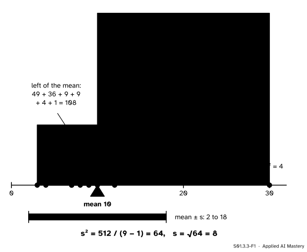
The obvious idea is to average the deviations from the mean. It fails at once: by S01.3.1 they always add up to zero, the negatives cancelling the positives. So remove the signs by squaring. Each squared deviation is the area of a square whose side is the deviation.
S01.3.3-F1
Every deviation drawn as a square. The squares add to 512, and the penthouse’s square alone is 400 of it. Spread out over \({9 - 1 = 8}\) and square-rooted, they give the standard deviation, 8.
The picture shows two things at once. First, squaring makes far values count far more: a value twice as far out contributes four times the area. Second, the penthouse dominates. Without it the other eight rents, measured from their own mean of 7.5, give squares that add to only 62. Like the mean it is built on, the standard deviation is not resistant.
The squares are in “hundreds of euros squared”, which means nothing to anyone. Taking the square root at the end brings the answer back to hundreds of euros: a typical distance from the mean, with far values weighted heavily.
Build it up
Step 1. Deviations. From the mean 10, the rents deviate by −7, −6, −3, −3, −2, −1, 0, 2, 20.
Step 2. Squares. Squaring gives 49, 36, 9, 9, 4, 1, 0, 4, 400. None is negative, so none can cancel another.
Step 3. Add. The sum of squares is 512.
Step 4. Divide by \({n - 1}\). With \({n = 9}\) the divisor is 8, and \({512 / 8 = 64}\). This is the variance, \(s^2\). The reason for 8 and not 9 is the subject of the formal section.
Step 5. Take the root.\({s = \sqrt{64} = 8}\), in hundreds of euros. This is the standard deviation. A band from \({{\bar{x} - s} = 2}\) to \({{\bar{x} + s} = 18}\) is a rough picture of where “most” of the rents lie, though for data this lopsided it is a poor one (lesson S01.3.4).
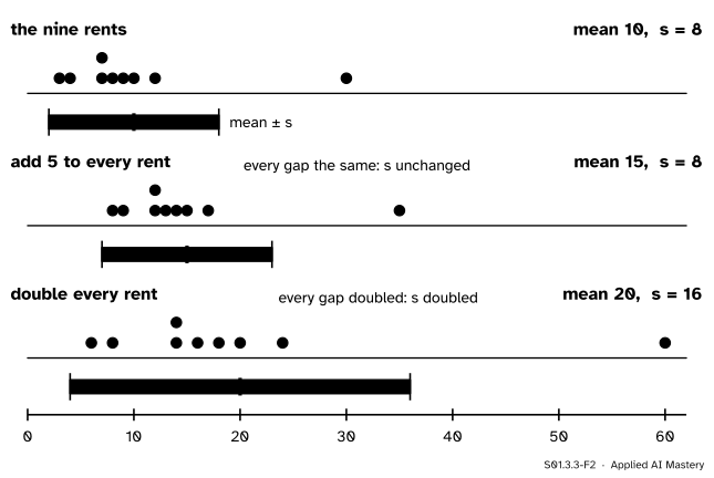
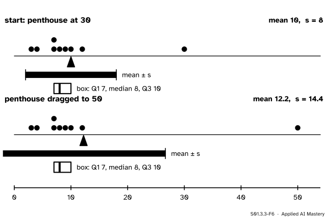
Step 6. Shift and stretch. Add the same amount to every rent and the dots slide together: no gap between them changes, so neither does the spread. Double every rent and every gap doubles, and so does the standard deviation.
S01.3.3-F2
A shift moves the mean and leaves \(s\) alone. A change of scale multiplies both the mean and \(s\).
The formal statement
NoteDefinitions: variance and standard deviation
For sample values \({x_1, \dots, x_n}\) with mean \(\bar{x}\), the variance and the standard deviation are
Result 1: shifts and changes of unit. Let \({y_i = a x_i + b}\) for numbers \(a\) and \(b\). By exercise 3 of S01.3.1, \({\bar{y} = a\bar{x} + b}\). So each new deviation is
\[
\begin{aligned}
y_i - \bar{y} &= (a x_i + b) - (a\bar{x} + b) \\
&= a\,(x_i - \bar{x}).
\end{aligned}
\]
The shift \(b\) has cancelled. Square and add, taking the constant \(a^2\) out of the sum:
Taking roots, \({s_y = \abs{a}\,s_x}\): a shift leaves the standard deviation alone, and a change of unit multiplies it by the size of the scale factor. In euros instead of hundreds of euros the standard deviation of the rents is 800 euros; with a charge of 50 euros added to every rent it is still 800 euros. The sign of \(a\) does not matter: turning every value round, \({y = -x}\), flips the picture but keeps every distance.
Result 2: why \({n - 1}\). The nine flats are a sample from the city (S01.2.1). What we would like is the city’s variance \(\sigma^2\), which measures the squared distances to the city’s mean \(\mu\). But \(\mu\) is unknown, so the formula measures distances to the sample’s own mean \(\bar{x}\) instead. Result 2 of S01.3.1, with \({c = \mu}\), compares the two:
The last term can never be negative, so a sample is always at least as close to its own mean as to \(\mu\), and usually closer. Squared deviations from \(\bar{x}\) therefore come up short, and dividing them by \(n\) falls short of \(\sigma^2\) on average. Dividing by the smaller number \({n - 1}\) makes up the difference exactly. The proof for every \(n\) needs expected values and is in S02.2; here is the smallest case, checked by listing every possibility.
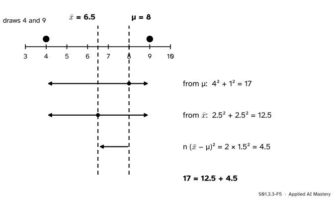
S01.3.3-F5
One draw of two from the five-flat population, rents 4 and 9. Measured from their own mean 6.5 the squares add to 12.5; measured from the population mean 8 they add to 17. The gap is \({{n\,(\bar{x} - \mu)^2} = 4.5}\).
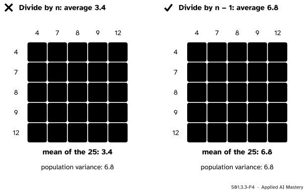
The check. S01.2 used a five-flat population with rents 4, 7, 8, 9 and 12: \({N = 5}\), \({\mu = 8}\), squared deviations adding to 34, so \({\sigma^2 = 34/5 = 6.8}\). Draw one flat, put it back, draw again: there are \({5 \times 5 = 25}\) equally likely ordered draws of two, and each gives a sample variance. Over all 25:
the squared distances to \(\mu\), \({\sum (x_i - \mu)^2}\), average \({13.6 = 2 \times 6.8}\), since each of the two draws runs through every flat equally often;
the gap \({n\,(\bar{x} - \mu)^2}\) averages \(6.8\), one variance’s worth;
so the squared distances to \(\bar{x}\) average \({{13.6 - 6.8} = 6.8}\).
Dividing that by \({n = 2}\) gives an average of 3.4, half the truth. Dividing by \({n - 1 = 1}\) gives exactly 6.8. A sample of \(n\) loses, on average, one variance’s worth of squared distance by being measured from its own mean, and the divisor \({n - 1}\) puts it back.
Go deeper: why the check uses draws with the flat put back
Without putting the first flat back there are only ten samples of two, and their variances average 4.25 with divisor \(n\) and 8.5 with divisor \({n - 1}\): now \({n - 1}\) overshoots. The cause is that a population of five is used up as it is sampled: having drawn the 12, you cannot draw it again, so the second draw is pushed towards the other side. A small sample from a large population, such as nine flats from a city of 500, behaves almost exactly like draws with the flat put back, and that is the setting of the proof in S02.2.
Go deeper: a shortcut for the sum of squares, and why programs avoid it
Expanding the squares gives \({\sum (x_i - \bar{x})^2} = {\sum x_i^2 - n\bar{x}^2}\). For the rents, \({1412 - 9 \times 100 = 512}\). It saves a pass through the data, but when the values are large and close together it subtracts two huge, nearly equal numbers and loses digits in floating point. NumPy and pandas compute the deviations first.
Worked example
The standard deviation of the nine rents, row by row.
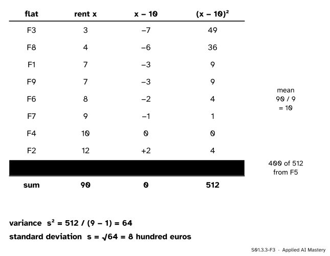
S01.3.3-F3
The calculation as a table: the mean first, then each deviation, then each square. The deviations add to 0, the squares to 512.
The mean is \({90 / 9 = 10}\).
The deviations are listed in the third column. They add to 0, which checks the mean.
The squares add to 512, and \({s^2 = 512 / 8 = 64}\).
The standard deviation is \({s = 8}\) hundred euros, or 800 euros.
Without the penthouse the mean is 7.5, the deviations are −4.5, −3.5, −0.5, −0.5, 0.5, 1.5, 2.5, 4.5, and their squares add to 62. So \({s^2 = 62 / 7 \approx 8.86}\) and \({s \approx 2.98}\). One flat out of nine multiplied the standard deviation by about 2.7.
Code
From scratch first, then the library calls, whose defaults differ.
import mathrents = [7, 12, 3, 10, 30, 8, 9, 4, 7] # F1 to F9, hundreds of euros a monthdef variance(values, divisor_offset=1):"""Sum of squared deviations from the mean, divided by n - divisor_offset.""" n =len(values) m =sum(values) / nreturnsum((x - m) **2for x in values) / (n - divisor_offset)s2 = variance(rents)s = math.sqrt(s2)eight = [r for r in rents if r !=30]print("variance", s2, " sd", s, " without the penthouse:", round(math.sqrt(variance(eight)), 2))print("in euros:", math.sqrt(variance([100* r for r in rents]))," plus 50 euros:", math.sqrt(variance([100* r +50for r in rents])))
variance 64.0  sd 8.0  without the penthouse: 2.98
in euros: 800.0  plus 50 euros: 800.0
Now every ordered draw of two from the five-flat population, with both divisors.
from itertools import productpopulation = [4, 7, 8, 9, 12]mu =sum(population) /len(population)sigma2 =sum((x - mu) **2for x in population) /len(population)draws =list(product(population, repeat=2)) # 25 ordered draws, the first flat put backby_n = [variance(d, divisor_offset=0) for d in draws]by_n_minus_1 = [variance(d) for d in draws]print(len(draws), "draws; population variance", sigma2)print("average with divisor n:", sum(by_n) /25, " with n - 1:", sum(by_n_minus_1) /25)
25 draws; population variance 6.8
average with divisor n: 3.4   with n - 1: 6.8
The libraries: NumPy divides by \(n\) unless told otherwise with ddof=1 (“delta degrees of freedom”: the divisor is \(n\) minus ddof). pandas divides by \({n - 1}\) unless told otherwise.
The same column, two libraries, two answers (7.54 and 8) unless you say which divisor you want.
Explore
S01.3-X1
Balance and middle
Drag the penthouse (F5) right, then left past the others, or choose a flat and use its slider or its \({-1}\) and \({+1}\) buttons. Watch which summaries follow a single value and which hold still, and turn on Deviations to see them cancel at every position.
Two things to try. Drag the penthouse from 30 to 50: the mean moves by \({20/9 \approx 2.22}\) and \(s\) jumps from 8 to about 14.4, while the median and the IQR do not move. Then bring the penthouse down to 5: now it sits among the cheap flats, the median falls to 7 and the quartiles become 5 and 9.
Pitfalls
S01.3.3-F4
Wrong beside right, over every possible sample of two. With the divisor \(n\) the sample variances average 3.4, half the population variance. With \({n - 1}\) they average 6.8 exactly.
“np.std gives the standard deviation of my sample.”
By default NumPy divides by \(n\), which is the population formula. For the rents np.std returns 7.54, not 8. Pass ddof=1 for a sample, and remember that pandas already does. When two programs give slightly different standard deviations for the same column, check this setting first.
“The standard deviation is the average distance from the mean.”
It is the root of the average squared distance, which weights far values more. The plain average distance of the rents from 10 is \({{44 / 9} \approx 4.89}\), well below \({s = 8}\), because the penthouse’s distance of 20 counts as 400 before the root is taken.
“Dividing by \({n - 1}\) makes every sample’s standard deviation right.”
It makes the variance right on average over all samples, not right for any one sample, and not right for the standard deviation. Over the 25 draws above, \(s^2\) averages 6.8, but \(s\) averages about 2.04 against \({\sigma = \sqrt{6.8} \approx 2.61}\): the square root of an average is not the average of the square roots. S02.2 returns to this.
Check yourself
Recall
1. What are the sum of squares, the variance and the standard deviation of the nine rents?
2. Why can you not measure spread by averaging the deviations from the mean?
Show answer
They always add to zero, so their average is zero for every data set.
3. If every value is changed to \({a x + b}\), what happens to the standard deviation?
Show answer
It is multiplied by \(\abs{a}\). The shift \(b\) has no effect.
4. For the 25 ordered draws of two from the population 4, 7, 8, 9, 12, what do the sample variances average with the divisor \(n\), and with \({n - 1}\)?
Show answer
3.4 with \(n\), and exactly 6.8, the population variance, with \({n - 1}\).
5. Which divisor do numpy.std and pandas.Series.std use by default?
Show answer
NumPy divides by \(n\) (ddof=0); pandas divides by \({n - 1}\) (ddof=1).
Exercises
1.★ The areas of the nine flats are 55, 75, 25, 60, 155, 70, 35, 30 and 35 square metres, with mean 60. Find their standard deviation.
Show solution
The deviations from 60 are −5, 15, −35, 0, 95, 10, −25, −30, −25, and they add to 0. Their squares are 25, 225, 1225, 0, 9025, 100, 625, 900 and 625, which add to 12,750. So \({s^2 = 12750 / 8 = 1593.75}\) and \({s = \sqrt{1593.75} \approx 39.9}\) square metres. As with the rents, the penthouse (155) contributes most of the sum: 9,025 of 12,750.
2.★★ Every rent rises by 5 percent and then a charge of 20 euros is added. Find the new standard deviation and the new variance, in hundreds of euros.
Show solution
The new rent is \({y = 1.05\,x + 0.2}\) in hundreds of euros. By Result 1, \({s_y = 1.05 \times 8 = 8.4}\), and the charge has no effect. The variance is \({s_y^2 = 1.05^2 \times 64 = 70.56}\), or equally \(8.4^2\).
3.★★★ Show that a sample of two values \(a\) and \(b\) has variance \({s^2 = (a - b)^2 / 2}\). Use it to explain why 5 of the 25 draws above have variance 0, and to find the largest variance among them.
Show solution
The mean is \({(a + b)/2}\). The two deviations are
Each squared is \({(a - b)^2/4}\), so the sum of squares is \({(a - b)^2/2}\), and with divisor \({n - 1 = 1}\) that is the variance. A draw has variance 0 exactly when \({a = b}\), which happens when the same flat is drawn twice: five of the 25 draws. The largest variance comes from the two flats furthest apart, 4 and 12: \({(12 - 4)^2 / 2 = 32}\), which appears twice, as (4, 12) and (12, 4).
Summary card
Square the deviations, add, divide by \({n - 1}\), take the root.
S01.3.3-F1
512 / 8 = 64, and \({\sqrt{64} = 8}\).
Variance.\(s^2 = {\frac{1}{n-1}\sum (x_i - \bar{x})^2}\); standard deviation\({s = \sqrt{s^2}}\).
Units.\({y = a x + b}\) gives \({s_y = \abs{a}\,s_x}\).
Why \({n - 1}\). Distances to \(\bar{x}\) fall short of distances to \(\mu\) by \({n(\bar{x} - \mu)^2}\).
Code.np.std(x, ddof=1); pandas uses \({n - 1}\) by default.
Sources and next steps
Sources. Each was opened and checked against this lesson on 12 November 2026.
David Diez, Mine Cetinkaya-Rundel and Christopher Barr, OpenIntro Statistics, 4th edition (free PDF). Section 2.1.4, Variance and standard deviation: the variance as the squared deviations added and divided by \({n - 1}\), the remark that dividing by \({n - 1}\) rather than \(n\) makes the statistic more reliable, and the standard deviation as its square root.
NIST/SEMATECH, e-Handbook of Statistical Methods, Section 1.3.5.6, Measures of scale: the variance with divisor \({N - 1}\), the standard deviation as its square root in the units of the data, and the warning that extreme values in the tails can distort the standard deviation.
NumPy documentation, numpy.var: the divisor is \(N\) minus ddof, with ddof=0 by default, and ddof=1 gives the sample variance, an unbiased estimate of the variance of a larger population (Bessel’s correction).
pandas documentation, Series.std: the sample standard deviation, normalised by \({N - 1}\) by default (ddof=1).