The same counts can call for the split comparison under one story and the pooled one under another. Learn the rule of time order, work Berkeley’s 1973 admissions, and simulate how a coin flip that assigns the treatment makes the reversal disappear.
Explain why one table of counts can call for the split comparison under one causal story and the pooled comparison under another.
Decide whether to split or pool by asking whether the third variable is settled before the treatment or is changed by it.
Read Berkeley’s 1973 admissions both ways and say which question each view answers.
Simulate a randomised experiment with a seeded generator and show that a coin flip balances the groups and removes the reversal.
In review. The maths and code on this page are checked by automated tests on every change, but an independent reader has not signed it off yet. Spot a mistake or a confusing step? Tell us.
The question
Take the kidney-stone table and change only its labels: column B is now a new drug, column A no drug, and the rows split patients by their blood pressure measured after treatment. Every count stays the same. In S01.7.3 the right answer came from the split rows. Is it still the split rows now, and if not, what tells you so, given that the numbers have not changed?
From the last lesson
1. What are the directly standardised success rates of A and B on the mix of all 700 patients?
Show answer
83.3% for A and 77.9% for B: each treatment’s two group rates averaged with the same weights, 357/700 and 343/700.
2. What makes a variable a confounder, at this level?
Show answer
It comes before the treatment, it influences which treatment a unit gets, and it influences the outcome by itself.
Intuition
Pearl, Glymour and Jewell tell the kidney-stone counts twice, as two different studies. Their point is that the table cannot tell the two studies apart, yet the two studies call for opposite answers.
S01.7.4-F1
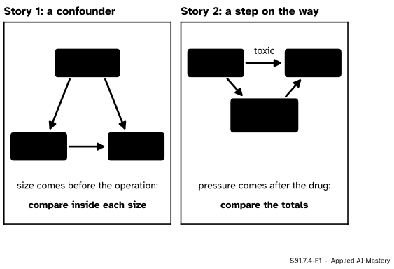
The same counts under two stories. In the first, the third variable comes before the treatment and acts on it; in the second, the treatment acts on the third variable.
Story 1, the confounder. Stone size is settled before any doctor chooses an operation, and it steers the choice. Comparing all A patients with all B patients compares hard cases with easy ones. Comparing inside each stone size removes that difference. Split.
Story 2, a step on the way. Now the third column is blood pressure measured after the drug. The drug lowers blood pressure, and low blood pressure helps recovery: 270 of the 350 patients on the drug ended with low pressure, against 87 of the 350 without it. The drug also has a small toxic effect, which is what shows inside each pressure level. Splitting by pressure compares patients the drug has already sorted, and so hides the benefit that works through pressure. To learn what taking the drug does, compare the totals: 82.6% recover on the drug against 78.0% without. Pool.
Nothing in the table tells the stories apart. The difference is the order of events, what can influence what: knowledge about the world, not about the numbers. As the primer puts it, no statistical method can determine the causal story from the data alone.
Build it up
Step 1. A real case: Berkeley, 1973. For graduate study at the University of California, Berkeley, 8,442 men and 4,321 women applied. The university admitted 44% of the men and 35% of the women. Was it biased against women?
Step 2. Split by department. Applicants apply to a department, and each department decides. In the six largest departments, 2,691 men and 1,835 women applied.
Dept
Men admitted
Women admitted
A
62% of 825
82% of 108
B
63% of 560
68% of 25
C
37% of 325
34% of 593
D
33% of 417
35% of 375
E
28% of 191
24% of 393
F
6% of 373
7% of 341
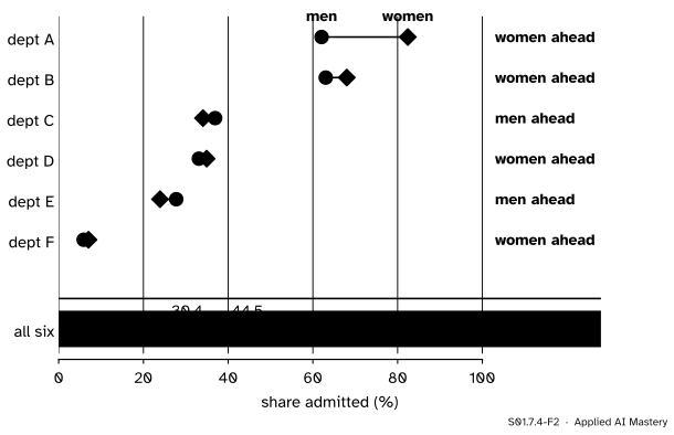
Across these six, 44.5% of the men and 30.4% of the women were admitted. Yet women were ahead in four of the six departments: A, B, D and F.
S01.7.4-F2
Berkeley’s six largest departments in 1973. Women were ahead in four departments and far behind when the six were pooled.
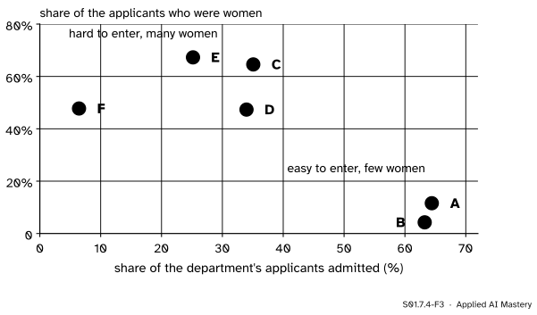
Step 3. Find the mix. The departments differed enormously in how hard they were to enter, and men and women applied to different ones. Over half the men (1,385 of 2,691) applied to A and B, which admitted about two thirds of their applicants. Only 7% of the women (133 of 1,835) did; most applied to C to F, which admitted about a third of their applicants or fewer.
S01.7.4-F3
Each department as one point. The departments that admitted few applicants were the ones women applied to.
Step 4. Which view answers which question? The department is chosen by the applicant before any decision is made, as stone size is settled before the operation. So “did departments treat men and women differently?” is a question for the split view, and in these six the answer is: not to women’s disadvantage. The pooled view answers another true question: “what share of the men and of the women who applied got in?”. Its gap is real, and it raises a question the table cannot answer: why were the departments that women chose so hard to enter?
The formal statement
NoteRule of time order (for one third variable)
To learn the effect of a treatment on an outcome, in a table split by a third variable:
if the third variable is settled before the treatment, and may influence it, compare within its groups (split, or standardise as in S01.7.3);
if the treatment can change the third variable, which then lies on the way to the outcome, compare the totals (pool).
The rule covers the simple stories of this module, with one third variable. With many variables the order of events is no longer enough, and course S06 gives the general answer with causal diagrams.
Randomisation cuts the arrow into the treatment. Suppose a coin, not a doctor, decides who gets A. The coin cannot see the stone, so stone size loses its arrow into the treatment, and with it the power to confound. In numbers: each arm then receives roughly the same mix of stones as the whole set of patients.
Look at the ideal case first, where the coin splits each stratum exactly in half. Then arm A gets \(n_g / 2\) of the \(n_g\) patients of stratum \(g\), out of \(n / 2\) patients in all, so its share of stratum \(g\) is
the share of the whole set, and the same holds for arm B. Each arm’s crude rate is its weighted mean with weights \(w_g\) (S01.7.1), and now those weights are the standard weights \(W_g\):
So the crude comparison is the standardised comparison, and by S01.7.1 it cannot reverse the comparison inside the strata. A real coin does not split each stratum exactly in half, but with many patients it comes close, as the simulation below shows. It does the same for confounders nobody recorded, which no standardisation can reach. That is why randomised experiments (S05.1) are the standard for learning effects.
Go deeper: Berkeley, standardised
Standardise the admission rates of men and women in the six departments to one shared mix: each department weighted by its total number of applicants, 933, 585, 918, 792, 584 and 714 (4,526 in all). The men’s rates give
and the women’s rates, with the same weights, give \(0.430\). On one shared mix of departments, women were admitted at 43.0% and men at 38.7%: the reversal of the pooled 30.4% against 44.5% is the kidney-stone reversal again, with departments as the strata.
Worked example
Simulate the study twice: once with the doctors choosing, once with a coin.
Make 100,000 patients with the study’s mix of stones: each has a small stone with chance 357/700. Give each operation its observed success rate for each stone size, so that, by design, A is better for both sizes. Then assign the operation in two ways. Doctors choose: a small stone gets A with chance 87/357, a large one with chance 263/343, as in the study. A coin chooses: every patient gets A with chance one half.
S01.7.4-F4
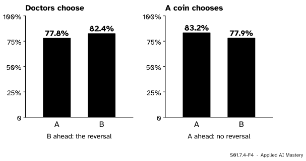
The trace of the simulation. When doctors choose, the arms get different mixes and the reversal appears; when a coin chooses, both arms get about 51% small stones and A is ahead.
Doctors choose. Arm A ends up with about 25% small stones and arm B with about 78%, close to the study’s 24.9% and 77.1%. The crude success rates are about 77.8% for A and 82.4% for B: the reversal is back, close to the study’s 78.0% and 82.6%.
A coin chooses. Both arms end up with about 51% small stones, the share of the whole set. The crude rates are about 83.2% for A and 77.9% for B, within a few tenths of a point of the standardised rates of S01.7.3, 83.3% and 77.9%. With a coin, the plain comparison of the two arms gives the right answer, with no table of strata needed.
These numbers depend on the seed: another seed moves them by a few tenths of a point, not enough to change the order.
Code
The simulation from scratch with a seeded NumPy generator: one array per column, and a comparison with a uniform random number to decide each event.
import numpy as nprng = np.random.default_rng(0)n =100_000small = rng.random(n) <357/700# the study's mix of stonesp_A = np.where(small, 81/87, 192/263) # success rates by designp_B = np.where(small, 234/270, 55/80)by_doctor = rng.random(n) < np.where(small, 87/357, 263/343)by_coin = rng.random(n) <0.5result = {}for design, gets_A in (("doctors choose", by_doctor), ("a coin chooses", by_coin)): success = rng.random(n) < np.where(gets_A, p_A, p_B) result[design] = (success[gets_A].mean(), success[~gets_A].mean(), small[gets_A].mean(), small[~gets_A].mean()) a, b, sa, sb = result[design]print(f"{design}: A {100* a:.1f}% ({100* sa:.0f}% small) B {100* b:.1f}% ({100* sb:.0f}% small)")
doctors choose: A 77.8% (25% small)  B 82.4% (78% small)
a coin chooses: A 83.2% (51% small)  B 77.9% (51% small)
Now Berkeley with pandas: the counts of the six departments in a DataFrame, the pooled and split rates with groupby, and the standardised rates with numpy.average.
import pandas as pdberkeley = pd.DataFrame({"dept": list("ABCDEF") *2,"sex": ["men"] *6+ ["women"] *6,"admitted": [512, 353, 120, 138, 53, 22, 89, 17, 202, 131, 94, 24],"applied": [825, 560, 325, 417, 191, 373, 108, 25, 593, 375, 393, 341],})pooled = berkeley.groupby("sex")[["admitted", "applied"]].sum()pooled_rate = pooled["admitted"] / pooled["applied"]split = berkeley.assign(rate=berkeley["admitted"] / berkeley["applied"]).pivot(index="dept", columns="sex", values="rate")dept_size = berkeley.groupby("dept")["applied"].sum()standardised = {s: float(np.average(split[s], weights=dept_size)) for s in ("men", "women")}print({s: round(float(v), 3) for s, v in pooled_rate.items()})print(split.round(2))print("women ahead in", int((split["women"] > split["men"]).sum()), "of 6 departments")print({s: round(v, 3) for s, v in standardised.items()})
{'men': 0.445, 'women': 0.304}
sex    men  women
dept
A     0.62   0.82
B     0.63   0.68
C     0.37   0.34
D     0.33   0.35
E     0.28   0.24
F     0.06   0.07
women ahead in 4 of 6 departments
{'men': 0.387, 'women': 0.43}
Explore
Go back to Split the scatter in S01.7.2 and set both gaps to zero. That is what randomisation does to a confounder: the course no longer shifts the hours or the scores, the between part vanishes, and the pooled line runs like the lines inside the courses. Move one gap only and the between part stays at zero: a confounder needs both of its arrows.
Pitfalls
S01.7.4-F5
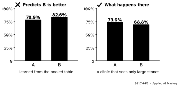
Wrong beside right. A rule learned from the pooled table recommends B; at a clinic whose patients all have large stones, A does better.
“Split by every variable you have; more detail is always safer.”
Not when the treatment changes the variable. Splitting the drug trial by blood pressure measured afterwards compares patients the drug had already sorted, and hides the drug’s main benefit. Ask of each variable whether it was settled before the treatment.
“Once the split view is right, the pooled numbers are wrong.”
Pooled numbers are correct descriptions: Berkeley really did admit 44% of its male and 35% of its female applicants. They answer a different question, and a report should say which question each figure answers.
“A model that fits the training data well has learned how the world works.”
A model trained on the pooled kidney table learns that patients given B succeed more often, an association that rests on the doctors’ mix of patients. At a clinic that treats only large stones its advice is wrong. This is dataset shift (E05.4): an association that rests on a mix of groups lasts only as long as the mix does.
Check yourself
Recall
1. In the blood-pressure story, which comparison gives the effect of the drug, and why?
Show answer
The totals (82.6% against 78.0%), because the drug changes blood pressure and part of its benefit works through it; splitting by pressure afterwards hides that benefit.
2. State the rule of time order.
Show answer
If the third variable is settled before the treatment, compare within its groups; if the treatment can change it, compare the totals.
3. What were Berkeley’s overall admission rates in 1973, and in how many of the six largest departments were women ahead?
Show answer
44% of 8,442 men and 35% of 4,321 women; women were ahead in four of the six (A, B, D and F).
4. Why does a coin flip remove confounding by stone size?
Show answer
The coin cannot see the stone, so stone size no longer influences the treatment; each arm gets about the same mix of stones, and the crude comparison becomes the standardised one.
5. Why can a model trained on pooled data fail after deployment?
Show answer
It learns the pooled association, which depends on the mix of groups in the training data; when the mix shifts, the association changes and the model’s advice can reverse.
Exercises
1.★ Split or pool? (a) Comparing two teaching methods by exam marks, with a table split by the students’ marks in the previous year. (b) Comparing two fertilisers by crop yield, with a table split by plant height measured at harvest, which the fertiliser affects. (c) Comparing two surgeons’ success rates, with a table split into easy and difficult operations, when the difficulty of a case is known before it is assigned to a surgeon.
Show solution
(a) Split: last year’s marks are settled before the teaching method and may have influenced who got which method. (b) Pool: the fertiliser changes plant height, which lies on the way to the yield. (c) Split: difficulty is settled before the case reaches a surgeon, and a surgeon who takes the difficult cases would look worse in the totals.
2.★★ In the coin-flip design, suppose the coin is replaced by a rule that gives A to exactly half of the small stones and exactly half of the large stones. Compute both arms’ crude success rates for the study’s 700 patients (round the half of 357 and 343 as you like, and let each operation keep its own rate for each stone size), and compare them with the standardised rates of S01.7.3.
Show solution
Each arm gets half of each stratum, so its share of small stones is \(357/700 = 0.510\), exactly as in the formal statement (rounding the halves moves the shares by less than 0.002). Each arm’s crude rate is then its weighted mean with the standard weights: A has \({0.510 \times 0.931} + {0.490 \times 0.730} = 0.833\) and B has \({0.510 \times 0.867} + {0.490 \times 0.688} = 0.779\), the standardised rates 83.3% and 77.9%. With balanced arms, crude and standardised comparisons agree.
3.★★★ In the drug story of the hook, compute the share of patients with low blood pressure afterwards on the drug and without it. Then show that if the drug had not changed blood pressure, so that both arms had the same share \(w\) of low pressure, the totals would favour no drug for every value of \(w\). Explain what this says about where the drug’s benefit comes from.
Show solution
On the drug (column B), \(270/350 = 77.1\%\) ended with low pressure; without it (column A), \(87/350 = 24.9\%\). If both arms had the same share \(w\) of low pressure, the difference of the totals would be
and both brackets are positive, so no drug (A) would be ahead for every \(w\) between 0 and 1, by between 4.3 and 6.4 points. The drug’s advantage in the totals, 82.6% against 78.0%, therefore comes entirely from moving patients into the low-pressure group, which is exactly the effect that splitting by pressure would hide.
Summary card
Split or pool depends on what causes what, and the table does not say.
S01.7.4-F1
Same counts, two stories.
Before the treatment (stone size, department): compare within groups or standardise.
Changed by the treatment (blood pressure afterwards): compare the totals.
Berkeley 1973. 44% of men and 35% of women admitted; women ahead in 4 of the 6 largest departments; standardised, 43.0% against 38.7%.
Randomise. A coin gives each arm the same mix, so the crude comparison is the fair one.
Sources and next steps
Sources. Each was opened and checked against this lesson on 12 November 2026.
Judea Pearl, Madelyn Glymour and Nicholas P. Jewell, Causal Inference in Statistics: A Primer, chapter 1 (the authors’ copy). Section 1.2: the same counts with post-treatment blood pressure in place of sex (Table 1.2, columns switched), where the aggregate data give the right answer, and the statement that no statistical method can determine the causal story from the data alone.
Wikipedia, Simpson’s paradox, section on UC Berkeley gender bias: 8,442 men and 4,321 women applied, 44% and 35% admitted, and the applicants and percentages admitted in the six largest departments, citing Bickel, Hammel and O’Connell, Science, 1975.
R documentation, UCBAdmissions: admissions to the six largest Berkeley departments in 1973, 4,526 applicants (2,691 men and 1,835 women), from Bickel, Hammel and O’Connell (1975). The admitted counts of the Code section are this data set’s.
Rafael A. Irizarry, Introduction to Data Science, chapter 19, Association is not causation. Section 19.4 works the six majors: 44% of men and 30% of women admitted, with women applying mostly to the more selective majors.
Next. S01.8, An analysis workflow from start to finish, puts the traps of this module into a full analysis. Randomised experiments are the subject of S05.1, and confounders and adjustment of S06.3.