A recorded value is a true value plus error: rounding, random scatter and a systematic offset. Separate the offset from the scatter by hand, see by simulation that averaging shrinks only the scatter, and ask whether a column measures what the question is about.
Write a recorded value as a true value plus error, and name three kinds of error: rounding, random and systematic.
Separate the offset from the scatter in a set of repeated readings, by hand and in code.
Show by a seeded simulation that averaging more readings shrinks the scatter and leaves the offset.
Judge whether a column is a valid stand-in for the quantity a question asks about, and apply the same test to labels in machine learning.
In review. The maths and code on this page are checked by automated tests on every change, but an independent reader has not signed it off yet. Spot a mistake or a confusing step? Tell us.
The question
A laser meter reads every floor 1.5 square metres too large. You measure one flat a hundred times and average. Is the answer now right? And when a dataset for machine learning carries a label typed in by a person, is that label the truth or one more measurement?
From the last lesson
1. What separates an interval scale from a ratio scale?
Show answer
On a ratio scale zero means none of the quantity; on an interval scale zero is a convention, so ratios of values make sense only on a ratio scale.
2. Under \(x \to ax + b\), what happens to the difference of two values?
Show answer
It becomes \({a(x_1 - x_2)}\): the shift cancels, so a ratio of two differences is unchanged.
Intuition
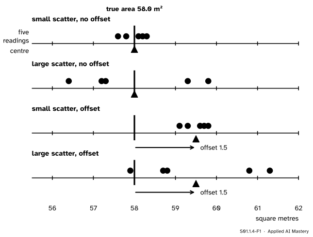
The 60 in F4’s area cell is not the floor itself. It is the end of a process: someone held a meter, read a number and wrote it down rounded. Each stage can add an error. Picture four meters, each used five times on a floor whose true area is 58.0 square metres.
S01.1.4-F1
Four meters, five readings each, of one floor of 58.0 m². Random error spreads the readings around their own centre. Systematic error moves the centre itself off the true value.
Two different things can go wrong, and the picture keeps them apart. The readings can scatter: each one lands somewhere different, for reasons nobody controls. And the whole cloud can be offset: every reading pushed the same way, so that their centre sits off the truth. A meter can have either problem, both, or neither. Lesson S01.2.2 will find the same two problems in samples, where the offset is called bias.
Build it up
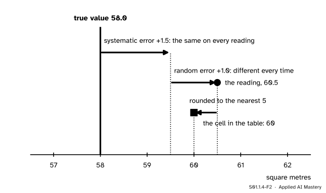
Step 1. A reading is the truth plus error. Take one reading of F4’s floor, 60.5 m². Split it into the parts that made it.
S01.1.4-F2
One reading taken apart. The truth, plus an offset that never changes, plus a random error that changes every time, gives the reading. Rounding gives the cell.
Step 2. Rounding. The table gives areas to the nearest 5 m², so the 60.5 reading is written as 60. Any reading between 57.5 and 62.5 would have been written as 60, so the rounding error is at most 2.5 either way.
Step 3. Random error. Measure again and the meter says 59.0, then 58.5. A random error is the part of the error that changes unpredictably from one reading to the next: a hand that wobbles, a beam that hits a skirting board.
Step 4. Systematic error. A systematic error is the part that stays the same on every reading, or changes in a predictable way: a meter that measures from the wrong end of its own case, a scale that is never set back to zero. Because it repeats, repeating the measurement can never reveal it. Only comparing with something whose true value is known can.
The formal statement
NoteDefinition: measurement error
The measurement error of a reading is the reading minus the true value. Over repeated readings of one quantity it splits into a systematic error\(\closs{\delta}\), the same every time, and a random error\(\closs{e_i}\) that changes unpredictably. Reading \(i\) of a true value \(\ctruth{v}\) is
These follow the definitions of the International Vocabulary of Metrology (entries 2.16, 2.17 and 2.19), which also calls an estimate of the systematic error the measurement bias (2.18).
What averaging does. Add up \(n\) readings, term by term:
\[
\begin{aligned}
\bar{x} &= v + \delta + \bar{e}, \\
\bar{x} - v &= \delta + \bar{e},
\end{aligned}
\]
where \(\bar{e}\) is the mean of the random errors. The random errors point both ways, so in a mean they partly cancel, and \(\bar{e}\) tends to get smaller as \(n\) grows; the code below shows how fast. The offset \(\delta\) is the same in every reading, so it survives into the mean whole. Averaging fights random error and does nothing to systematic error.
What rounding does to a mean. Let \(r_i\) be value \(i\) after rounding to the nearest 5, so each rounding error \(r_i - x_i\) lies between \(-2.5\) and \(2.5\). The mean of the rounded values minus the mean of the unrounded ones is
an average of numbers between \(-2.5\) and \(2.5\), so it lies between \(-2.5\) and \(2.5\) too. The mean area of the table, 60 m², is within 2.5 m² of the mean of the unrounded areas.
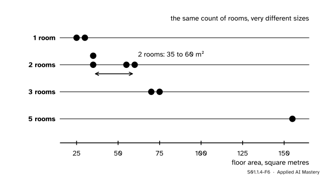
Validity: does the column measure the right thing? A column can be read perfectly and still answer the wrong question. If the question is how big the flats are, rooms is a tempting stand-in for size, since it is easy to count.
S01.1.4-F6
Rooms as a stand-in for size. The four two-room flats run from 35 to 60 m²: a reliable count, but a rough measure of the quantity the question is about.
A measure is valid for a question when it captures the quantity the question asks about. Rooms is counted without error, but F7 and F4 both have two rooms and differ by 25 m². Reliability (getting the same reading again) and validity (reading the right thing) are separate virtues. Jacobs and Wallach (2021) carry both ideas into machine learning, where unobservable quantities such as socioeconomic status or the risk of reoffending are inferred through measurable stand-ins.
Worked example
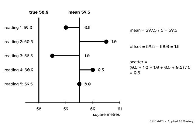
Five readings of F4’s floor, whose plans give 58.0 m², are 59.0, 60.5, 58.5, 60.0 and 59.5. Separate the offset from the scatter. (The readings and the plans are invented for this lesson.)
S01.1.4-F3
The worked example. The offset is the distance from the truth to the centre of the readings; the scatter is the average distance of the readings from their own centre.
The centre. The readings add to \(59.0 + 60.5 + 58.5 + 60.0 + 59.5 = 297.5\), so their mean is \(297.5 / 5 = 59.5\).
The offset. The centre minus the true value: \(59.5 - 58.0 = 1.5\). The meter reads about 1.5 m² too high. Five readings cannot say exactly how much of the 1.5 is the meter’s \(\delta\) and how much is \(\bar{e}\), the average of this time’s random errors; a reading of something whose area is known would settle it.
The scatter. The distance of each reading from 59.5 is 0.5, 1.0, 1.0, 0.5 and 0.0. Their average is \(3.0 / 5 = 0.6\). This average distance from the centre is the measure of scatter used until S01.3 introduces the standard deviation.
The cell. Rounded to the nearest 5, every one of these readings, and their mean, is written as 60. The cell hides both the offset and the scatter.
Code
The worked example from scratch.
true_area =58.0readings = [59.0, 60.5, 58.5, 60.0, 59.5]def mean(values):returnsum(values) /len(values)def scatter(values):"""The average distance of the values from their own mean.""" centre = mean(values)returnsum(abs(v - centre) for v in values) /len(values)def nearest_5(x):return5*round(x /5)print("mean:", mean(readings), " offset:", mean(readings) - true_area, " scatter:", round(scatter(readings), 2))print("as written in the table:", sorted({nearest_5(r) for r in readings}))
mean: 59.5   offset: 1.5   scatter: 0.6
as written in the table: [60]
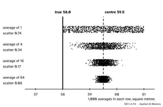
Now a meter with a known offset of 1.5 and random errors anywhere from \(-1.5\) to \(1.5\), drawn with a seeded generator. For each \(n\), the simulation takes 1,000 averages of \(n\) readings and reports their centre and their scatter.
import numpy as nprng = np.random.default_rng(0)offset =1.5results = {}for n in (1, 4, 16, 64): sim = true_area + offset + rng.uniform(-1.5, 1.5, size=(1000, n)) averages = sim.mean(axis=1) results[n] = (averages.mean(), np.mean(np.abs(averages - averages.mean())))print(f"n = {n:2d}: centre {results[n][0]:.2f} scatter {results[n][1]:.2f}")
n =  1: centre 59.55   scatter 0.74
n =  4: centre 59.48   scatter 0.34
n = 16: centre 59.51   scatter 0.17
n = 64: centre 59.50   scatter 0.08
S01.1.4-F4
The simulation drawn. Each time the number of readings is multiplied by four, the scatter of the averages roughly halves. The centre stays at 59.5, 1.5 above the truth, however many readings go in.
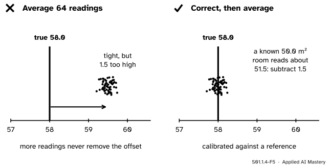
The scatter falls from about 0.74 to 0.34, 0.17 and 0.08: roughly halving each time \(n\) is quadrupled, a law that M06.11.1 and S02.1 derive. The centre stays within 0.06 of 59.5 every time. The offset does not shrink at all. One cure works: measure something whose true value is known, a test room of exactly 50.0 m², learn the offset, and subtract it.
The estimate is 1.36, not exactly 1.5: it is itself an average of 64 readings, so it carries a little random error of its own. The corrected average, 58.17, is within 0.2 of the truth, where the uncorrected averages sat 1.5 too high.
Explore
The module’s interactive, the Scale ladder, is in lesson S01.1.3. Choose area and change the unit to square feet: every statement survives, because a change of unit re-expresses a measurement without altering it. The errors of this lesson are different: no change of unit can remove them.
Pitfalls
S01.1.4-F5
Wrong beside right. Averages of 64 readings are tight but still 1.5 too high. Measuring a known area first finds the offset, and subtracting it moves the averages onto the truth.
“With enough readings, the errors average out.”
Only the random ones. The derivation shows \(\bar{x} - v = \delta + \bar{e}\): more readings shrink \(\bar{e}\) and leave \(\delta\) untouched. The same holds for data in machine learning: more rows shrink the noise in an estimate, but if every row was measured the same wrong way, a million rows learn the same wrong thing (E05.3).
“The readings agree closely, so the meter is accurate.”
Agreement measures scatter, not offset. The third meter in the anchor figure puts every reading within half a square metre of their centre, and that centre is 1.5 m² too high. Close agreement says the meter is precise; only a comparison with a known value says it is right.
“The label column is the ground truth.”
A label is a measurement made by a person or a process, and it carries the same errors. Northcutt, Athalye and Mueller (2021) estimated an average of at least 3.3 percent label errors across the test sets of ten widely used benchmarks, and at least 6 percent in the ImageNet validation set. A label can also be a poor stand-in, like rooms for size: what was easy to record instead of what the question is about.
Check yourself
Recall
1. Write a reading as the sum of its parts.
Show answer
\(x_i = v + \delta + e_i\): the true value, plus a systematic error that is the same every time, plus a random error that changes from reading to reading.
2. What does averaging more readings do to each kind of error?
Show answer
It shrinks the random error in the average, because random errors partly cancel. It leaves the systematic error unchanged, because every reading carries all of it.
3. The table gives areas to the nearest 5 m². How far can a recorded area be from the reading it came from, and how far can the mean of the recorded areas be from the mean of the readings?
Show answer
At most 2.5 m² in each case: every rounding error lies between \(-2.5\) and \(2.5\), and so does their average.
4. For the five readings 59.0, 60.5, 58.5, 60.0 and 59.5 of a true 58.0, what are the offset and the scatter?
Show answer
The mean is 59.5, so the offset is 1.5. The distances from 59.5 are 0.5, 1.0, 1.0, 0.5 and 0.0, so the scatter is 0.6.
5. What is the difference between a reliable measure and a valid one?
Show answer
A reliable measure gives the same reading when repeated. A valid one captures the quantity the question asks about. Rooms is reliable but a weak measure of size.
Exercises
1.★ A kitchen scale weighs a 500 g reference weight four times: 507, 503, 506 and 504 g. Find the offset and the scatter, and say what you would do before weighing anything else.
Show solution
The readings add to 2020, so the mean is 505 g and the offset is \(505 - 500 = 5\) g. The distances from 505 are 2, 2, 1 and 1, so the scatter is \(6/4 = 1.5\) g. Before weighing anything else, subtract 5 g from each reading (or reset the scale); averaging several readings will then also shrink the 1.5 g scatter.
2.★★ Each of the nine flats’ areas was rounded to the nearest 5 m², and the recorded mean is 60 m². What can you say about the mean of the unrounded areas? Could it be 63?
Show solution
Each rounding error lies between \(-2.5\) and \(2.5\), and the difference of the two means is the average of the nine rounding errors, so it too lies between \(-2.5\) and \(2.5\). The mean of the unrounded areas lies between 57.5 and 62.5 m². It cannot be 63.
3.★★★ A spam filter is trained on messages labelled by users who press “report spam”. Name a random error and a systematic error this label could carry, and say which one more training data would reduce.
Show solution
A random error: a user clicks the button by accident on a wanted message now and then, or forgets to report a spam message, in no fixed pattern. A systematic error: users never report the newsletters they once signed up for and no longer read, so a whole kind of unwanted message is always labelled “not spam”. Also a validity problem: “reported by a user” stands in for “is spam”, and the two differ. More data of the same kind dilutes the random clicks, whose effect partly cancels, but every new row carries the same systematic error, so the filter keeps learning that unread newsletters are wanted. Only a better measurement, such as a careful relabelling of a sample, finds and corrects it.
Summary card
A recorded number is the truth plus error, and only part of the error averages away.
S01.1.4-F1
Scatter around the centre; offset of the centre.
Reading:\(x_i = v + \delta + e_i\), then rounded for the table (error at most half the step).
Offset = mean of readings minus true value; scatter = average distance from their mean.
Averaging shrinks scatter (about half for four times the readings) and keeps the offset.
Calibration against a known value finds the offset; nothing else does.
Validity: a reliable column can still measure the wrong thing. Labels are measurements too.
Sources and next steps
Sources. Each was opened and checked against this lesson on 12 November 2026.
Joint Committee for Guides in Metrology, International vocabulary of metrology (VIM), JCGM 200:2012, 3rd edition. Entry 2.16 defines measurement error as the measured value minus a reference value; 2.17 systematic error as the component that remains constant or varies predictably in replicate measurements, with a note that a correction can compensate a known systematic error; 2.18 measurement bias as an estimate of a systematic error; 2.19 random error as the component that varies unpredictably.
Curtis G. Northcutt, Anish Athalye and Jonas Mueller, Pervasive Label Errors in Test Sets Destabilize Machine Learning Benchmarks, NeurIPS 2021 Datasets and Benchmarks Track. The abstract estimates at least 3.3 percent label errors on average across ten test sets and at least 6 percent in the ImageNet validation set.
Abigail Z. Jacobs and Hanna Wallach, Measurement and Fairness, ACM FAccT 2021. Unobservable theoretical constructs are operationalised through measurement models, judged by construct reliability and construct validity.
NumPy documentation, Generator.uniform: samples are uniformly distributed over the half-open interval from low to high.