Divide the covariance by both standard deviations and you get Pearson’s r: a number with no units that lies between -1 and 1. Learn it as the average product of z-scores, prove its range, and meet the trend line whose slope it sets.
Compute Pearson’s r as the covariance over both standard deviations, and as the sum of products of z-scores over n - 1.
Prove that r has no units and does not change under a shift or a positive rescaling of either column.
Prove that r lies between -1 and 1, and say when it reaches either end.
State the slope and intercept of the trend line, and tell the strength of a relationship apart from its slope.
In review. The maths and code on this page are checked by automated tests on every change, but an independent reader has not signed it off yet. Spot a mistake or a confusing step? Tell us.
The question
The covariance of area and rent was 306.25 with rent in hundreds of euros and 30,625 with rent in euros, for the same nine flats. Is either number large? Neither can say. What number measures how closely two columns move together, the same in every unit, so that the link between area and rent can be set beside the link between any two other columns? Machine learning asks this whenever it screens features against a target or looks for two features that carry the same information.
From the last lesson
1. A point lies above and to the left of the point of means. What is the sign of its product of deviations?
Show answer
Negative: its \(x\)-deviation is negative and its \(y\)-deviation positive.
2. What happens to the covariance \(s_{xy}\) when every \(x\) is changed to \({a x + b}\)?
Show answer
It becomes \({a\,s_{xy}}\): the shift cancels and the factor multiplies every product.
Intuition
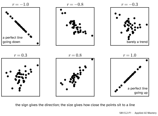
Covariance mixed two things: how the columns move together, and how big their units are. Strip out the units and only the first is left. The result is the correlation coefficient\(r\), also called Pearson’s \(r\). It always lies between \(-1\) and \(1\).
S01.5.2-F1
Six clouds and their correlations. The sign of \(r\) gives the direction; its size gives how closely the points keep to a straight line.
Read the six clouds from the outside in. At \(r = 1\) and \(r = -1\) every point lies on one straight line. As \(r\) moves towards \(0\) the cloud fattens, until at \(0\) it has no tilt at all. The sign is the direction from the last lesson; the size is new, and it measures strength: how tightly the points hug a line.
Build it up
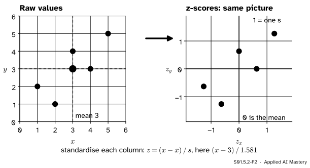
Step 1. Put both columns on the same scale. Replace every value by its z-score from S01.3.4, \(z = {(x - \bar{x}) / s}\): how many standard deviations it sits from its mean. For the five points, \(x = 1, \dots, 5\) and \(y = 2, 1, 4, 3, 5\), both means are \(3\) and both standard deviations are \(\sqrt{2.5} = 1.581\).
S01.5.2-F2
Standardising moves the origin to the point of means and measures each axis in its own standard deviations. The shape of the cloud is untouched.
Step 2. Multiply in pairs. The product \({z_{x,i}\,z_{y,i}}\) has the same sign as the rectangle of the last lesson, because each z-score is a deviation divided by a positive number. What has gone is the unit: both factors are pure numbers.
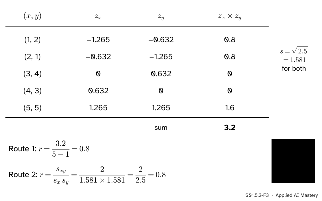
Step 3. Average. Add the products and divide by \(n - 1\). That average is \(r\). For the five points the products are \(0.8, 0.8, 0, 0, 1.6\), which add to \(3.2\), and \({3.2 / 4} = 0.8\).
The formal statement
NoteDefinition: Pearson’s correlation coefficient
For two columns whose standard deviations \(s_x\) and \(s_y\) are not zero,
Property 1: no units.\(s_{xy}\) carries the unit of \(x\) times the unit of \(y\); \(s_x\) and \(s_y\) carry one each. They cancel, so \(r\) is a pure number.
Property 2: a shift or a positive rescaling leaves \(r\) alone. Change \(x\) to \(u = {a x + b}\). The last lesson showed \(s_{uy} = {a\, s_{xy}}\), and S01.3.3 showed \(s_u = {\abs{a}\, s_x}\). So
For \(a > 0\) the fraction \({a / \abs{a}}\) is \(1\) and \(r\) does not move: rent in euros or in hundreds, area in square metres or square feet, the correlation is the same. For \(a < 0\) it is \(-1\), and \(r\) only flips its sign. The same holds for \(y\), since \(r\) treats its two columns alike.
Property 3: \(-1 \le r \le 1\). First a fact about z-scores. Their squares add to \(n - 1\), because the squared deviations add to \({(n - 1)\, s_x^2}\) by the definition of \(s_x\):
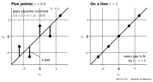
and the same for \(y\). Now take the gap \({z_{x,i} - z_{y,i}}\) between the two z-scores of each row. A sum of squares cannot be negative, so multiply out the square and use the fact:
Since \(2(n-1)\) is positive, \({1 - r \ge 0}\), which is \(r \le 1\). The same steps with the sum \({z_{x,i} + z_{y,i}}\) in place of the gap give \(0 \le {2(n-1)(1 + r)}\), which is \({r \ge -1}\) (Exercise 3).
S01.5.2-F4
The proof drawn. The squared gaps between \(z_y\) and \(z_x\) add to \({2(n-1)(1-r)}\). Gaps exist, so \(r < 1\); no gaps at all is the only way to reach \(r = 1\).
When \(r\) reaches \(1\) or \(-1\). The chain above shows \(r = 1\) exactly when every gap is zero: \(z_{y,i} = z_{x,i}\) for every row. Unwrap the z-scores:
a straight line with positive slope. Likewise \(r = -1\) exactly when the points lie on a straight line with negative slope. Anything short of a perfect line gives \({-1 < r < 1}\).
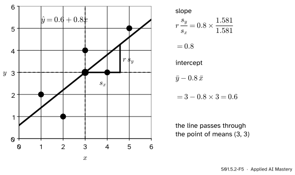
The trend line. The straight line that best follows a cloud, scored by squared vertical misses, is the least-squares line, or trend line. It passes through the point of means and its slope is
This lesson states it; ML01.4.2 derives it. Read the slope in two parts: one standard deviation across moves the line \(r\) standard deviations up. M06.10 gives the version of \(r\) for random variables.
S01.5.2-F5
The trend line of the five points: through \((3, 3)\), slope \(0.8\), intercept \(0.6\).
Worked example
The five points, both ways. The z-scores of \(x\) are the deviations \(-2, -1, 0, 1, 2\) divided by \(1.581\); those of \(y\) are \(-1, -2, 1, 0, 2\) divided by \(1.581\).
S01.5.2-F3
Pearson’s \(r\) for the five points by both routes: the average product of z-scores, and the covariance over the two standard deviations.
Route 1 multiplies the z-scores in pairs. Each product is a product of deviations divided by \(2.5\), so the products are \({2 / 2.5} = 0.8\), \(0.8\), \(0\), \(0\) and \({4 / 2.5} = 1.6\). They add to \(3.2\), and \(r = {3.2 / 4} = 0.8\).
Route 2 starts from the last lesson’s \(s_{xy} = 2\) and the standard deviations \(s_x = s_y = \sqrt{2.5}\):
\[
r = \frac{2}{\sqrt{2.5}\,\sqrt{2.5}} = \frac{2}{2.5} = 0.8 .
\]
The nine flats. Area has standard deviation \(s_x = 39.92\) square metres and rent \(s_y = 8\) hundred euros, so
\[
r = \frac{306.25}{39.92 \times 8} = 0.96 .
\]
With rent in euros, the covariance is \(30{,}625\) and \(s_y = 800\), and the quotient is again \(0.96\). The trend line has slope \({0.9589 \times 8 / 39.92} = 0.1922\) hundred euros per square metre, about 19 euros a month for each extra square metre, and intercept \({10 - 0.1922 \times 60} = -1.53\). (An intercept is where the line would cross zero area; no flat has zero area, so it is not a rent to read.)
Code
From scratch: z-scores, products, an average.
import mathdef mean(values):returnsum(values) /len(values)def sd(values): # divisor n - 1, as in S01.3.3 m = mean(values)return math.sqrt(sum((v - m) **2for v in values) / (len(values) -1))def pearson(x, y): zx = [(v - mean(x)) / sd(x) for v in x] zy = [(v - mean(y)) / sd(y) for v in y]returnsum(a * b for a, b inzip(zx, zy)) / (len(x) -1)x5, y5 = [1, 2, 3, 4, 5], [2, 1, 4, 3, 5]area = [55, 75, 25, 60, 155, 70, 35, 30, 35] # the flats table (invented)rent = [7, 12, 3, 10, 30, 8, 9, 4, 7]r5, r_flats = pearson(x5, y5), pearson(area, rent)w = r_flats * sd(rent) / sd(area)print("five points:", round(r5, 4), " flats:", round(r_flats, 4))print("rent in euros:", round(pearson(area, [100* v for v in rent]), 4))print("negated area:", round(pearson([-a for a in area], rent), 4))print("trend line: slope", round(w, 3), " intercept", round(mean(rent) - w * mean(area), 2))
five points: 0.8   flats: 0.9589
rent in euros: 0.9589
negated area: -0.9589
trend line: slope 0.192  intercept -1.53
The library calls give the same numbers. numpy.corrcoef returns a matrix with \(1\) on the diagonal (each column with itself) and \(r\) off it; DataFrame.corr does the same for every pair of columns at once.
import numpy as npimport pandas as pdprint(np.corrcoef(x5, y5))flats = pd.DataFrame({"area": area, "rent": rent})print(flats.corr().round(4))slope, intercept = np.polyfit(x5, y5, 1) # the least-squares line, for checkingprint("five points' line:", round(slope, 6), round(intercept, 6))
[[1.  0.8]
 [0.8 1. ]]
        area    rent
area  1.0000  0.9589
rent  0.9589  1.0000
five points' line: 0.8 0.6
Explore
This module’s interactive, the Anscombe explorer, lives in lesson S01.5.3. Drag points there and watch \(r\) and the trend line respond: pull one point far off the line and see how far one point can move \(r\).
Pitfalls
S01.5.2-F6
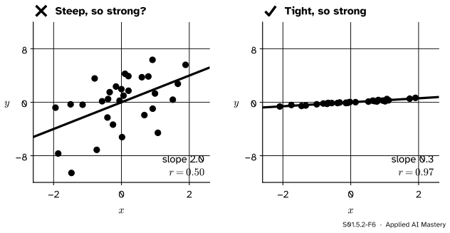
Wrong beside right. The steep cloud has the weak correlation; the flat one has the strong correlation. Strength is how tightly the points hug the line, not how steep the line is.
“A steeper trend line means a stronger correlation.”
The slope is \({r\, s_y / s_x}\): it has units and grows when \(y\) is spread more widely. \(r\) has no units and measures closeness to a line. A cloud can be steep and loose (slope 2, \(r = 0.5\)) or flat and tight (slope 0.3, \(r = 0.97\)). Only at \(r = 0\) do the two agree: the slope is then \(0\) too.
“\(r = -0.8\) is weaker than \(r = 0.5\).”
The sign is the direction, not the strength. \(r = -0.8\) keeps as close to a falling line as \(r = 0.8\) keeps to a rising one, and closer than \(r = 0.5\) keeps to its line.
“\(r = 0.8\) means 80 percent of the points are on the line.”
\(r\) is an average product of z-scores, not a share of points. In the five points none lies on the trend line \({\hat{y} = 0.6 + 0.8x}\), and still \(r = 0.8\).
Check yourself
Recall
1. Write \(r\) in two ways: with z-scores, and with the covariance.
Show answer
\(r\) is the sum of \({z_{x,i}\, z_{y,i}}\) divided by \(n - 1\), and it equals \({s_{xy} / (s_x s_y)}\).
2. What is \(r\) for the five points, and what is their covariance?
Show answer
\(r = 0.8\); the covariance is \(s_{xy} = 2\), and \({2 / 2.5} = 0.8\).
3. Between which values does \(r\) lie, and when does it reach the ends?
Show answer
Between \(-1\) and \(1\). It is \(1\) exactly when the points lie on a rising straight line and \(-1\) exactly when they lie on a falling one.
4. The rents are converted from hundreds of euros to euros. What happens to \(r\)? What if area is replaced by its negative?
Show answer
Nothing: a positive rescaling leaves \(r\) alone. Negating a column flips the sign of \(r\) and keeps its size.
5. State the slope and the intercept of the trend line.
Show answer
Slope \(w = {r\, s_y / s_x}\) and intercept \(b = {\bar{y} - w\,\bar{x}}\), so the line passes through the point of means.
Exercises
1.★ Two columns have \(s_{xy} = 12\), \(s_x = 4\) and \(s_y = 5\). Find \(r\) and the slope of the trend line.
Show solution
\(r = {12 / (4 \times 5)} = {12 / 20} = 0.6\). The slope is \({0.6 \times 5 / 4} = 0.75\): one unit across moves the line \(0.75\) up.
2.★★ In an invented record of 30 days, the correlation between the midday temperature in degrees Celsius and ice creams sold is \(0.7\). What is the correlation with the temperature in Fahrenheit, \(F = {1.8\,C + 32}\)? And with “degrees below 30 C”, that is \(30 - C\)?
Show solution
Fahrenheit is \({a C + b}\) with \(a = {1.8 > 0}\), so \(r\) is unchanged: \(0.7\). “Degrees below 30” is \({-1 \times C + 30}\), with \(a = {-1 < 0}\), so \(r\) flips sign: \(-0.7\). In both cases the cloud has the same shape; only the second is mirrored left to right.
3.★★★ Finish the proof of Property 3: show that \({r \ge -1}\), and that \(r = -1\) only when the points lie on a falling straight line.
Show solution
A sum of squares cannot be negative. Multiply out \({(z_{x,i} + z_{y,i})^2}\) and use that each set of squared z-scores adds to \(n - 1\):
Correlation is covariance with the units divided away.
S01.5.2-F1
Sign is direction; size is strength.
Definition.\(r = {s_{xy} / (s_x s_y)}\), the average product of z-scores with divisor \(n - 1\).
No units. A shift or a positive rescaling leaves \(r\) alone; a negative one flips its sign.
Range.\(-1 \le r \le 1\), with the ends only for points on a straight line.
Trend line. Slope \({r\, s_y / s_x}\), through \({(\bar{x}, \bar{y})}\); five points: \({\hat{y} = 0.6 + 0.8x}\).
Sources and next steps
Sources. Each was opened and checked against this lesson on 12 November 2026.
Allen B. Downey, Think Stats, third edition, Chapter 7. Section 7.3 computes Pearson’s correlation by standardising both columns and averaging the products of the standard scores; Section 7.4 notes that it measures the strength of a linear relationship.
David Diez, Mine Cetinkaya-Rundel and Christopher Barr, OpenIntro Statistics, fourth edition (free PDF). Section 8.1, fitting a line, residuals and correlation, at the level of this course.
NumPy developers, numpy.corrcoef, NumPy 2.5 reference. It returns \(R_{ij} = {C_{ij} / \sqrt{C_{ii} C_{jj}}}\) from the covariance matrix \(C\), with values between \(-1\) and \(1\).