A comparison that reverses: Simpson’s paradox in a table
Open surgery beats a keyhole operation for small kidney stones and for large ones, yet loses overall. See why: an overall rate is a weighted mean of group rates, and the two treatments were averaged with very different weights.
Compute success rates inside each group and overall from a table of counts, and spot a reversal between them.
Derive that an overall rate is the weighted mean of the group rates, with each group’s share of the patients as its weight.
Explain Simpson’s paradox as two weighted means taken with different weights, and show that equal weights cannot reverse a comparison.
Build the rates and the shares of a two-way table from scratch and with pandas.crosstab and groupby.
In review. The maths and code on this page are checked by automated tests on every change, but an independent reader has not signed it off yet. Spot a mistake or a confusing step? Tell us.
The question
Two operations remove kidney stones. Open surgery, call it A, succeeds more often than a closed, keyhole operation, call it B, for patients with small stones. It also succeeds more often for patients with large stones. Yet across all 700 patients, B succeeds more often than A. How can all three statements be true at once, and which operation should a doctor pick?
Intuition
The numbers come from a real study. In 1986 Charig and colleagues compared operations for kidney stones: A was open surgery and B was percutaneous nephrolithotomy, a keyhole operation through the skin. In 1994 Julious and Mullee laid out the counts below in a short paper on confounding. The same counts are the opening example of Pearl, Glymour and Jewell’s primer on causal inference. Each patient had one operation and the operation either worked or it did not. The patients are split by the size of their stone, small or large.
S01.7.1-F1
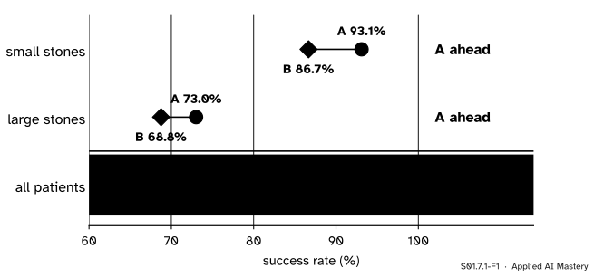
The kidney-stone study. Inside each stone size the blue circle (A) is to the right of the sky-blue diamond (B). Across all patients the order flips. Nothing has been miscounted.
A wins in both groups and loses overall. This is Simpson’s paradox: a comparison that holds inside every group reverses when the groups are pooled. It is named after Edward Simpson, who wrote about it in 1951, though others had noticed it before him.
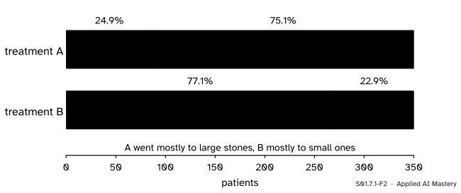
It is not a trick of the arithmetic, and it is not rare. The whole explanation fits in one sentence: A was mostly given to the hard cases. Large stones are harder to remove for either operation, and three quarters of A’s patients had large stones. B’s patients were mostly the easy cases. An overall rate mixes the easy and the hard cases together, so it reports the mix as much as the operation.
The same thing happens in machine learning. Two models scored on two test sets, one full of hard examples and one full of easy ones, can swap places in a table of accuracies while one of them is better on every kind of example.
Build it up
Step 1. The counts. Each cell holds successes over patients.
Stones
Treatment A
Treatment B
small
81 / 87
234 / 270
large
192 / 263
55 / 80
all
273 / 350
289 / 350
The bottom row adds the two rows above it: 81 + 192 = 273 successes from 87 + 263 = 350 patients for A, and 234 + 55 = 289 from 270 + 80 = 350 for B. Both treatments had 350 patients.
Step 2. Rates inside each group. A rate here is successes divided by patients. Inside one cell it is a conditional proportion, as in S01.5.4: the share of successes among the A patients with small stones, 81 / 87 = 93.1%. The four group rates are 93.1% and 73.0% for A, and 86.7% and 68.8% for B. A is ahead by 6.4 points for small stones and by 4.3 points for large ones (before rounding the large-stone rates are 73.00% and 68.75%).
Step 3. Rates overall. For all patients, A has 273 / 350 = 78.0% and B has 289 / 350 = 82.6%. B is ahead by 4.6 points.
Step 4. Who got which operation. Now look not at the successes but at the patients.
S01.7.1-F2
The mix of each treatment’s patients. A’s bar is three quarters large stones; B’s bar is three quarters small stones.
Three quarters of A’s patients had large stones, and three quarters of B’s had small ones. Doctors chose the operation, and the choice depended on the stone. Large stones are also harder to remove: for both operations together, 247 of the 343 large stones were removed successfully (72.0%), against 315 of the 357 small ones (88.2%).
So A’s overall rate is dragged down by its many hard cases, and B’s is lifted by its many easy ones. The next section turns that sentence into an exact formula.
The formal statement
Take one treatment and split its \(n\) patients into groups \(g = 1, 2\) (small and large stones). Group \(g\) has \(n_g\) patients and \(s_g\) successes, so its rate is \(p_g = s_g / n_g\) and its share of the patients is \(\cparam{w_g} = n_g / n\). The shares are positive and add to 1, because \(n_1 + n_2 = n\).
NoteResult: an overall rate is a weighted mean
The overall rate \(\cmodel{p} = s / n\) is the weighted mean of the group rates, with the shares as weights:
Derivation. The successes of the whole treatment are the successes of its groups added up. A group’s successes are its patients times its rate, \(s_g = n_g\, p_g\), which is the definition of \(p_g\) multiplied through by \(n_g\). So
The third line splits one fraction into two. This is the weighted mean of S01.2.3, where the population mean was the stratum means weighted by the stratum shares; here the strata are stone sizes.
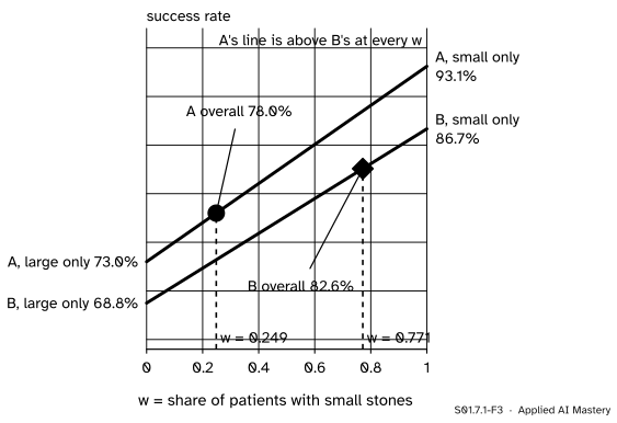
The overall rate is a point on a line. Write \(w\) for the share of small stones, so that the share of large stones is \({1 - w}\). Then
As \(w\) runs from 0 to 1, the overall rate runs in a straight line from \(p_2\) (large stones only) to \(p_1\) (small stones only). It always lies between the two group rates, and it sits nearer the rate of the bigger group.
S01.7.1-F3
Every possible overall rate of each treatment, one for each mix \(w\). A’s line is above B’s everywhere, but A sits far to the left (few small stones) and B far to the right.
Why the comparison reverses. Give the two treatments the superscripts A and B. Each has its own line, and A’s line is above B’s at every \(w\), because A is better for small stones and for large ones. But each treatment’s overall rate is read off its line at its own mix: A at \(w^{\text{A}} = 87 / 350 = 0.249\) and B at \(w^{\text{B}} = 270 / 350 = 0.771\). A low point on the higher line can be below a high point on the lower line.
With one shared mix, no reversal is possible. Suppose both treatments had the same share \(w\) of small stones. Subtract B’s weighted mean from A’s and group the terms by stone size:
If A is ahead in both groups, both brackets are positive. Their weights \(w\) and \({1 - w}\) are not negative and add to 1, so the sum is positive: A is ahead overall too. A reversal therefore needs two ingredients: the groups must differ in their rates (large stones are harder), and the treatments must differ in their mix (A got more large stones). Remove either one and the paradox disappears.
Go deeper: how many small stones would A have needed?
A’s overall rate at mix \(w\) is \({p_2^{\text{A}} + w\,(p_1^{\text{A}} - p_2^{\text{A}})}\). Setting this equal to B’s actual overall rate \(289/350\) and solving for \(w\):
So if just under half of A’s patients, instead of a quarter, had had small stones, A’s overall rate would have matched B’s 82.6%, even though B kept its easy mix of 77% small stones. Any share of small stones above 0.476 would have put A ahead overall.
Worked example
Rebuild both overall rates from the group rates and the shares.
S01.7.1-F4
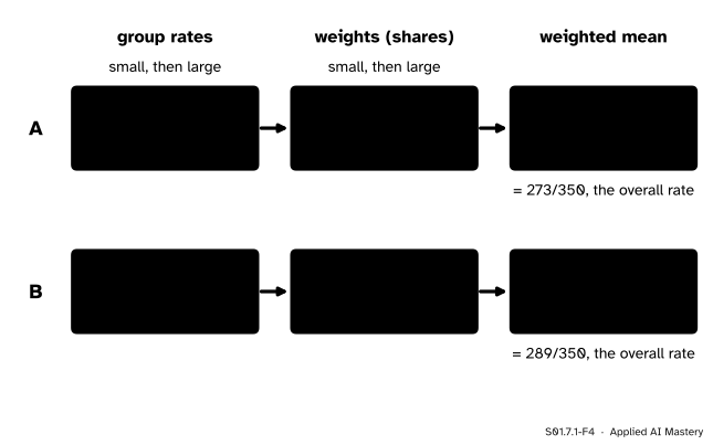
The trace of the worked example: group rates, then shares, then the weighted mean, which lands on the overall rate read straight from the table.
Treatment A. The group rates are \(81/87 = 0.931\) and \(192/263 = 0.730\). The shares are \(87/350 = 0.249\) and \(263/350 = 0.751\). The weighted mean is
That is the 273 / 350 of the table. It is no coincidence, and the rounding can be avoided altogether: each product is a share times a rate, and the group size cancels.
That is \(289/350\). Read the two sums side by side. Most of A’s weight, 0.751, sits on its lower rate, 0.730. Most of B’s weight, 0.771, sits on its higher rate, 0.867. A’s better rates cannot make up for that.
Code
First from scratch: the counts in a dictionary, the rates and shares by division, and the weighted mean as a sum.
counts = { # (successes, patients) for each treatment and stone size"A": {"small": (81, 87), "large": (192, 263)},"B": {"small": (234, 270), "large": (55, 80)},}summary = {}for treatment, groups in counts.items(): n =sum(patients for _, patients in groups.values()) rates = {size: s / m for size, (s, m) in groups.items()} shares = {size: m / n for size, (_, m) in groups.items()} overall =sum(shares[size] * rates[size] for size in groups) # the weighted mean summary[treatment] = (rates, shares, overall)print(treatment, {k: round(100* v, 1) for k, v in rates.items()},"shares", {k: round(v, 3) for k, v in shares.items()}, "overall", round(100* overall, 1))
A is ahead inside both groups and behind overall, and the weighted mean lands exactly on the overall rate. Now with pandas. A table of counts is a summary of one row per patient, so first rebuild those 700 rows, then let pandas.crosstab and groupby count them again.
import pandas as pdrows = []for treatment, groups in counts.items():for size, (s, m) in groups.items(): rows += [(treatment, size, 1)] * s + [(treatment, size, 0)] * (m - s)patients = pd.DataFrame(rows, columns=["treatment", "size", "success"])# The mean of a 0/1 column is a rate. margins=True adds the "All" column: the overall rate.rates = pd.crosstab(patients["treatment"], patients["size"], values=patients["success"], aggfunc="mean", margins=True)shares = pd.crosstab(patients["treatment"], patients["size"], normalize="index")print(patients.shape)print(rates.round(3))print(shares.round(3))print(patients.groupby(["treatment", "size"])["success"].mean().round(3))
(700, 3)
size       large  small    All
treatment
A          0.730  0.931  0.780
B          0.688  0.867  0.826
All        0.720  0.882  0.803
size       large  small
treatment
A          0.751  0.249
B          0.229  0.771
treatment  size
A          large    0.730
           small    0.931
B          large    0.688
           small    0.867
Name: success, dtype: float64
The All row of the rate table gives 72.0% for large stones and 88.2% for small ones: large stones are harder for everyone, which is half of the explanation. The share table, made with normalize="index" so that each row adds to 1, is the other half.
Explore
This module’s interactive, Split the scatter, lives in the next lesson, where the same reversal happens to a trend line. Before you go, try the formula by hand: give treatment B the mix of treatment A (24.9% small stones) and compute B’s overall rate. You should get 73.2%, now below A’s 78.0%. Lesson S01.7.3 turns that move into a method.
Pitfalls
S01.7.1-F5
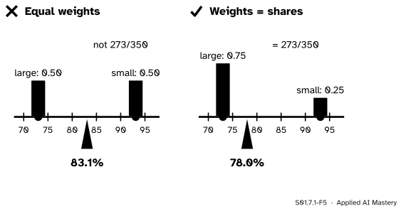
Wrong beside right, for treatment A. The overall rate is the balance point of the two group rates when each carries its share of the patients, not the midpoint between them.
“The overall rate is the average of the group rates.”
Only when the groups are the same size (or happen to have the same rate). The plain average of A’s rates, 93.1% and 73.0%, is 83.1%, but A’s overall rate is 78.0%, because three quarters of its patients sit in the group with the lower rate. Weight each group rate by its share of the patients.
“With more patients the reversal would go away.”
Multiply every count in the table by 100 and every rate and every share stays exactly the same, so the reversal stays too. Simpson’s paradox is not chance in a small sample. It comes from the mix, and more data drawn the same way keep the same mix.
“One of the two comparisons must be a mistake.”
Both are correct arithmetic and answer different questions. The group rates compare the operations on similar patients. The overall rates compare the two groups of patients who happened to get each operation, hard cases and all. Which question you should ask is the subject of S01.7.3 and S01.7.4. The same care applies when a leaderboard compares models evaluated on different test sets.
Check yourself
Recall
1. In the kidney-stone table, what are the success rates of A and B for small stones, for large stones and overall?
Show answer
Small: A 93.1%, B 86.7%. Large: A 73.0%, B 68.8%. Overall: A 78.0%, B 82.6%. A is ahead in each group and behind overall.
2. Write a treatment’s overall rate in terms of its group rates.
Show answer
\(p = w_1 p_1 + w_2 p_2\), where \(w_g = n_g / n\) is group \(g\)’s share of the treatment’s patients.
3. What share of A’s patients and what share of B’s patients had small stones?
Show answer
\(87/350 = 24.9\%\) for A and \(270/350 = 77.1\%\) for B.
4. Name the two ingredients that a reversal needs.
Show answer
The groups must differ in their rates (large stones are harder for both operations), and the treatments must differ in their mix of groups (A got more large stones).
5. If both treatments had the same mix of stones, could A be ahead in both groups and behind overall?
Show answer
No. With a shared weight \(w\), the overall difference is \(w\) times the small-stone difference plus \({1 - w}\) times the large-stone difference, and two positive differences with weights that are not negative give a positive sum.
Exercises
1.★ Two hospitals treat mild and severe cases of an illness (invented counts, recoveries over patients). Hospital P: mild 95 / 100, severe 120 / 300. Hospital Q: mild 270 / 300, severe 35 / 100. Compute the four group rates and the two overall rates. Is there a reversal?
Show solution
Mild: P 95%, Q 90%. Severe: P 40%, Q 35%. P is ahead in both groups. Overall: P has \((95 + 120)/400 = 215/400 = 53.75\%\) and Q has \((270 + 35)/400 = 305/400 = 76.25\%\). Q is ahead overall, so yes, the comparison reverses. P treated mostly severe cases (300 of 400), Q mostly mild ones.
2.★★ For hospital P of exercise 1, write the overall rate as a weighted mean and check it. Then find the share of mild cases P would need for its overall rate to equal Q’s 76.25%.
Show solution
P’s shares are \(100/400 = 0.25\) mild and \(300/400 = 0.75\) severe, so its overall rate is \({0.25 \times 0.95} + {0.75 \times 0.40} = 0.2375 + 0.30 = 0.5375\), which is 53.75%. With a share \(w\) of mild cases, P’s overall rate is \({0.40 + w\,(0.95 - 0.40)} = 0.40 + 0.55\,w\). Setting this equal to \(0.7625\) gives \(0.55\,w = 0.3625\), so \(w = 0.659\): about two thirds of P’s patients would have to be mild cases.
3.★★★ Prove that a weighted mean of group rates always lies between the smallest and the largest group rate, for any number of groups. Explain why this means the overall rate can never fall outside the range of the group rates.
Show solution
Let the groups have rates \(p_1, \dots, p_k\) and weights \(w_1, \dots, w_k\) that are not negative and add to 1. Write \(m\) for the smallest rate and \(M\) for the largest, so \(m \le p_g \le M\) for every \(g\). Multiplying by \(w_g \ge 0\) keeps the order: \(w_g m \le w_g p_g \le w_g M\). Adding over all groups, and using that the weights add to 1,
\[
\begin{aligned}
\textstyle\sum_g w_g p_g &\ge m \textstyle\sum_g w_g = m, \\
\textstyle\sum_g w_g p_g &\le M \textstyle\sum_g w_g = M .
\end{aligned}
\]
So \(m \le \sum_g w_g p_g \le M\). The overall rate is such a weighted mean with \(w_g = n_g / n\), so it lies between the smallest and the largest group rate. Simpson’s paradox never pushes an overall rate outside its own groups; it only places two treatments at different points of their own ranges.
Summary card
An overall rate is a weighted mean of group rates, and different weights can reverse a comparison.
S01.7.1-F1
Ahead in each group, behind overall.
Group rate.\(p_g = s_g / n_g\), successes over patients inside group \(g\).
Share.\(w_g = n_g / n\), the weight of group \(g\); the shares add to 1.
Overall rate.\(p = w_1 p_1 + w_2 p_2\), which lies between \(p_1\) and \(p_2\).
The paradox. Two treatments’ overall rates use their own shares. With one shared mix, no reversal is possible.
Sources and next steps
Sources. Each was opened and checked against this lesson on 12 November 2026 (the abstract of Charig and others on 14 November 2026).
Judea Pearl, Madelyn Glymour and Nicholas P. Jewell, Causal Inference in Statistics: A Primer, chapter 1 (the authors’ copy). Section 1.2 defines Simpson’s paradox as an association in a whole population that is reversed in every subpopulation, and its Table 1.1 has the counts of this lesson (81/87, 234/270, 192/263, 55/80, 273/350 and 289/350), told there as a drug trial split by sex.
Wikipedia, Simpson’s paradox, section on the kidney stone treatment. It gives the same table with treatments A and B and stone sizes small and large, and attributes the counts to Charig, Webb, Payne and Wickham (British Medical Journal,
and to Julious and Mullee, “Confounding and Simpson’s paradox” (BMJ, 1994).
C. R. Charig, D. R. Webb, S. R. Payne and J. E. Wickham, “Comparison of treatment of renal calculi by open surgery, percutaneous nephrolithotomy, and extracorporeal shockwave lithotripsy”, British Medical Journal volume 292, pages 879 to 882, abstract on PubMed: 350 patients had open surgery and 350 percutaneous nephrolithotomy, with success in 273 (78%) and 289 (83%) of them.
pandas documentation, pandas.crosstab: values with aggfunc, margins adding an All row and column, and normalize="index" making each row add to 1.
Next.S01.7.2 Simpson’s paradox in a scatter plot finds the same reversal in a trend line, where a correlation is positive inside every group and negative when the groups are pooled.