Filling every hole with the mean keeps all the rows and the mean, but it shrinks the spread by a factor you can compute, pulls correlations towards zero and plants a spike in the histogram. Derive each cost, soften them with group means and an indicator column, and fit the fill on training rows only.
Fill holes with the mean, the median or the most frequent value, and say which suits which column.
Derive that mean imputation keeps the mean and multiplies the variance by (n_obs - 1) / (n - 1).
Show that mean imputation shrinks a correlation and plants a spike in the histogram, and compute both on small data.
Explain how a group-mean fill and a was-missing indicator soften the damage, and why the fill value is learned from training rows only.
In review. The maths and code on this page are checked by automated tests on every change, but an independent reader has not signed it off yet. Spot a mistake or a confusing step? Tell us.
The question
A model needs a number in every cell, and deleting rows throws data away. So fill each hole with the column’s mean: every row survives and the mean does not move. It sounds free. What does it cost the spread of the column, its histogram and its correlation with every other column, and can you put a number on each cost?
From the last lesson
1. Ten independent columns each miss \(10\%\) of their values. What share of rows survives listwise deletion?
Show answer
\(0.9^{10} = 0.349\), about \(35\%\).
2. Why do df["rent"].mean() after dropna() and after dropna(subset=["rent"]) differ on the flats table with holes?
Show answer
Plain dropna() also drops F9, whose year is missing although its rent is known. The two means rest on six and seven rows: \(10.67\) and \(10.14\).
Intuition
Imputation means filling each hole with a value. The simplest kind, single imputation, fills each hole once with one number: the mean of the values seen, their median, or, for a category, the most frequent label. Every row is kept.
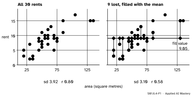
The trouble is that every hole in a column gets the same guess. Look at thirty invented flats, area against rent, after nine rents went missing at random and were filled with the mean of the twenty-one that remained.
S01.6.4-F1
Mean imputation on the thirty flats. The nine filled rents (diamonds) sit on one flat line at \(9.05\), however large or small the flat. The spread falls from \(3.92\) to \(3.10\) and the correlation of area with rent from \(0.80\) to \(0.58\).
Three costs show at once. The filled values add no spread, since each sits exactly at the mean. They add no relationship, since a large flat and a small flat get the same rent. And they pile up in one spot, which no real column would do.
Build it up
Step 1. Choose a fill. The mean suits a roughly symmetric number column; the median suits a skewed one, such as rents with a penthouse (S01.3.4); the most frequent value is the only one a category allows (S01.1.2), so a missing energy rating would become C.
Step 2. The mean stays. Filling with the mean of the values seen adds values equal to that mean, so the mean of the filled column is the same number.
Step 3. The spread shrinks. The variance adds up squared distances from the mean. Each filled value is at distance \(0\), so it adds nothing to the sum, yet it counts in the divisor.
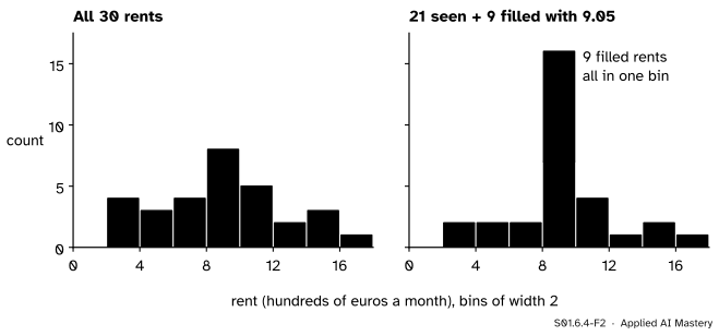
Step 4. The histogram grows a spike. All the filled values land in the bin that holds the mean.
S01.6.4-F2
The spike. The nine filled rents all fall in the bin from \(8\) to \(10\), which jumps to \(16\), twice the tallest bar of the complete data.
Step 5. Fill by group instead. If the rows fall into groups that differ, such as districts, fill each hole with the mean of its own group. A Centre flat then gets a Centre rent, and the filled values keep the differences between groups, so less spread is lost. A related idea records the fact of filling: a was-missing indicator column holds \(1\) where a value was filled and \(0\) elsewhere, so the analyst, and a model, can tell guesses from measurements.
The formal statement
Let a column have \(n\) rows, \(n_{\text{obs}}\) of them seen, with mean \(\bar{x}_{\text{obs}}\), and fill the other \({n - n_{\text{obs}}}\) with \(\bar{x}_{\text{obs}}\).
2. The variance is scaled down. Write \(SS\) for the sum of squared deviations of the values seen from \(\bar{x}_{\text{obs}}\). The filled values add \(0\) to it, so the filled column has the same \(SS\) but divides by \({n - 1}\):
With \(30\%\) of a long column filled, the variance drops to about \(70\%\) of that of the values seen.
3. The correlation is pulled towards zero. Let a second column \(x\) be complete, with mean \(\bar{x}\) over all rows, and let \(y\) be filled. Write \(O\) for the rows where \(y\) was seen, with means \(\bar{x}_O\) and \(\bar{y}_O\). A filled row has \({y_i - \bar{y}_O} = 0\), so it adds nothing to the sum of products, and over \(O\) the deviations \({y_i - \bar{y}_O}\) sum to zero, which lets \(\bar{x}\) be swapped for \(\bar{x}_O\):
The second line is the sum of products of the pairs seen. The sum of squares of \(y\) is also that of the values seen, while the sum of squares of \(x\), \(SS_x\), runs over all \(n\) rows. Dividing as in S01.5.2, with \(r_O\) the correlation of the pairs seen and \(SS_{x,O}\) the sum of squares of \(x\) over \(O\) about \(\bar{x}_O\),
The square root is at most \(1\): \(SS_x\) adds squares over more rows than \(SS_{x,O}\), and taken about \(\bar{x}_O\), the mean of the rows in \(O\), their squares are as small as they can be (S01.3.1). So filling can only shrink a correlation.
4. A group-mean fill gives the reweighted mean. Fill each hole in group \(g\) with \(\bar{x}_g\), the mean of the values seen in that group. Group \(g\)’s total becomes \(n_g \bar{x}_g\), so the mean of the filled column is \({\sum_g (n_g/n)\,\bar{x}_g}\), the reweighted mean of S01.6.2. Under MAR by group it has no lean; the plain mean fill does.
S01.6.4-F4
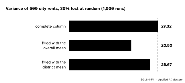
Filling with the district mean keeps most of the spread (\(26.67\) against \(29.32\)), because it keeps the differences between districts; the overall mean, at \(20.50\), keeps only about \(70\%\).
Worked example
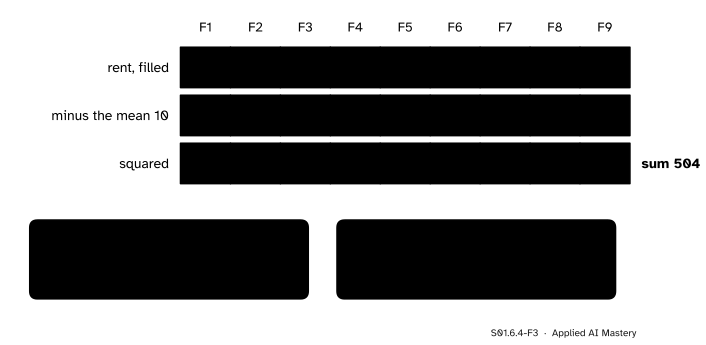
The nine rents with \(8\) and \(12\) hidden, filled with the mean. The seven rents seen are \(3, 4, 7, 7, 9, 10, 30\): sum \(70\), mean \(10\). Fill F2 and F6 with \(10\).
S01.6.4-F3
The same sum of squares, \(504\), divided two ways. The filled values add zeros to the sum but count in the divisor, so the variance falls from \(84\) to \(63\).
Mean. The filled column sums to \({70 + 10 + 10} = 90\), mean \({90/9} = 10\): unchanged.
Variance. The deviations of the rents seen from \(10\) square to \(49, 36, 9, 9, 1, 0, 400\), sum \(504\). The rents seen have variance \({504/6} = 84\). The filled column has variance \({504/8} = 63\), which is \({84 \times 6/8}\), as the formula says. Its standard deviation is \({\sqrt{63}} = 7.94\), below the \(9.17\) of the rents seen.
Correlation with area. The seven pairs seen have \(r_O = 0.979\). Area is complete, with \(SS_x = 12{,}750\) over all nine flats and \(SS_{x,O} = 12{,}335.7\) over the seven (about their own mean, \(56.4\)). So \(r_{\text{filled}} = {0.979 \times \sqrt{12335.7/12750}} = {0.979 \times 0.984} = 0.963\). The shrink is small here because the two flats filled have middling areas.
Group-mean fill. By district, South’s rents seen are \(3\) and \(4\) (mean \(3.5\)) and Centre’s are \(30\) and \(9\) (mean \(19.5\)). Filling F6 with \(3.5\) and F2 with \(19.5\) gives a column whose mean is \({\tfrac13(3.5 + 8 + 19.5)} = 10.33\), the reweighted mean, and whose variance is \(79.4\). The group fill kept, and here overshot, the spread: one Centre flat stood in for its district and its guess, \(19.5\), is far from the hidden \(12\). Over many runs on the city it lands close, as the figure in the formal section shows.
Code
From scratch: fill, then measure what changed.
import numpy as nparea = np.array([55, 75, 25, 60, 155, 70, 35, 30, 35], dtype=float)rent = np.array([7, 12, 3, 10, 30, 8, 9, 4, 7], dtype=float)seen =~np.isin(rent, [8, 12]) # 8 and 12 are hiddenfilled = np.where(seen, rent, rent[seen].mean())ss = ((rent[seen] - rent[seen].mean()) **2).sum()print("SS", ss, " var seen", ss / (seen.sum() -1), " var filled", filled.var(ddof=1))r_seen = np.corrcoef(area[seen], rent[seen])[0, 1]factor = np.sqrt(((area[seen] - area[seen].mean()) **2).sum() / ((area - area.mean()) **2).sum())print(f"r seen {r_seen:.3f} x factor {factor:.3f} = {r_seen * factor:.3f}; r filled {np.corrcoef(area, filled)[0, 1]:.3f}")district = np.array(["North", "Centre", "South", "North", "Centre", "South", "Centre", "South", "North"])by_group = filled.copy()for g in ("South", "North", "Centre"): inside = district == g by_group[inside &~seen] = rent[inside & seen].mean()print("group fill:", by_group, " mean", round(by_group.mean(), 2), " var", round(by_group.var(ddof=1), 1))
SS 504.0  var seen 84.0  var filled 63.0
r seen 0.979  x factor 0.984 = 0.963;  r filled 0.963
group fill: [ 7.  19.5  3.  10.  30.   3.5  9.   4.   7. ]  mean 10.33  var 79.4
The identity \({r_{\text{filled}}} = {r_O \times \text{factor}}\) holds exactly. Now the city: \(30\%\) of the rents lost at random, \(1{,}000\) times, filled with the overall mean and with the district mean.
rng = np.random.default_rng(0) # the city of course S01parts, names = [], []for name, size, mu in (("South", 250, 5.0), ("North", 150, 8.0), ("Centre", 100, 17.0)): draws = rng.gamma(9.0, 1.0, size) parts.append(draws * mu / draws.mean()) names += [name] * sizecity, names = np.concatenate(parts), np.array(names)rng = np.random.default_rng(2)plain_var, group_var = [], []for _ inrange(1000): hole = rng.random(500) <0.3 a = np.where(hole, city[~hole].mean(), city) g = city.copy()for name in ("South", "North", "Centre"): inside = names == name g[inside & hole] = city[inside &~hole].mean() plain_var.append(a.var(ddof=1)) group_var.append(g.var(ddof=1))print(f"complete {city.var(ddof=1):.2f} overall-mean fill {np.mean(plain_var):.2f} district fill {np.mean(group_var):.2f}")
complete 29.32 overall-mean fill 20.50 district fill 26.67
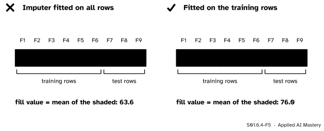
In machine learning the fill value is a parameter learned from data, so it is learned from the training rows only and then applied unchanged to new rows (ML01.2.4). scikit-learn’s SimpleImputer does this, and add_indicator=True appends the was-missing column. Here F1 to F6 are the training rows and F7 to F9 the test rows; F4 and F7 have no area.
from sklearn.impute import SimpleImputertrain = np.array([[55], [75], [25], [np.nan], [155], [70]]) # F1 to F6test = np.array([[np.nan], [30], [35]]) # F7 to F9imputer = SimpleImputer(strategy="mean", add_indicator=True).fit(train)print("learned fill value:", imputer.statistics_)print(imputer.transform(test)) # area, then the was-missing column
learned fill value: [76.]
[[76.  1.]
 [30.  0.]
 [35.  0.]]
The test flat F7 gets \(76\), the mean of the five training areas, and not \(63.6\), the mean of every area seen, which would let the test rows shape their own fill. strategy="median" and strategy="most_frequent" give the other two fills.
Explore
Open the missingness machine in lesson S01.6.2 and press Fill with the mean. Lose rents at random and push the slider up: the read-out shows the standard deviation and \(r\) falling together as more diamonds line up on the mean. Then lose high rents: the fill keeps the mean of what is left, so it keeps that mean’s lean as well.
Pitfalls
S01.6.4-F5
Wrong beside right. Fitted on every row, the fill value uses the test rows’ areas. Fitted on the training rows, it is \(76.0\), and the test rows are filled with that.
“After filling, the column is complete, so its summaries are real.”
The mean may be right, but the standard deviation is too small by the factor of the formal section, and every correlation is shrunk. Report how many values were filled, and compute spreads and correlations from the values seen.
“The fill value is just cleaning, so I compute it on the whole table.”
A fill value is learned from data, like a scaler’s mean. Computed on all rows, it lets the test rows leak into training, the first leak of ML01.2.4. Fit the imputer on the training rows and apply it to the rest.
“Filling repairs the bias of missing data.”
A mean fill keeps the mean of the values seen, bias included: under MNAR the filled column is as far off as the rows that survived. The indicator column does not cure it either: van Buuren shows the indicator method can bias a regression badly even under MCAR. Proper repairs, which add back the uncertainty of each guess, are the multiple imputation of S08.7.
Check yourself
Recall
1. Which simple fill suits a skewed number column, and which suits a category?
Show answer
The median for a skewed number column; the most frequent value for a category.
2. By what factor does mean imputation multiply the variance?
Show answer
\({(n_{\text{obs}} - 1)/(n - 1)}\), because the filled values add nothing to the sum of squares but count in the divisor.
3. On the nine rents with \(8\) and \(12\) hidden, what is the variance before and after filling?
Show answer
\({504/6} = 84\) for the seven rents seen, and \({504/8} = 63\) after filling with \(10\).
4. Why can mean imputation only shrink a correlation?
Show answer
\(r_{\text{filled}} = {r_O \sqrt{SS_{x,O}/SS_x}}\), and \({SS_{x,O} \le SS_x}\) because the sum over all rows has more squares and the rows seen are measured about their own mean, which makes their squares as small as possible.
5. What is the mean of a column filled with group means?
Show answer
The reweighted mean \({\sum_g (n_g/n)\,\bar{x}_g}\) of lesson S01.6.2, with \(\bar{x}_g\) the mean of the values seen in group \(g\).
Exercises
1.★ A column has \(50\) rows, \(40\) seen, with variance \(25\). What is the variance after mean imputation, and the standard deviation before and after?
Show solution
\({25 \times 39/49} = 19.90\). The standard deviation falls from \({\sqrt{25}} = 5\) to \({\sqrt{19.90}} = 4.46\).
2.★★ The ratings of the nine flats are C, B, D, B, A, C, D, C, C. The ratings of F2 and F7 are lost and filled with the most frequent of the seven seen. What fill is used, and how do the counts of the four ratings change?
Show solution
F2 (B) and F7 (D) are lost, leaving C, D, B, A, C, C, C: four C, one each of A, B and D. The most frequent is C, so both holes become C. The counts go from A 1, B 2, C 4, D 2 to A 1, B 1, C 6, D 1: the spike is now in the C bar, and B and D each lose one.
3.★★★ Show that filling with any single constant \(c\) instead of the mean gives a filled column whose variance is at least that of the mean-filled column.
Show solution
Write \(a = \bar{x}_{\text{obs}}\), \(d = {c - a}\) and \(q = {(n - n_{\text{obs}})/n}\), the share filled. The filled column \(y\) has the values seen plus \({n - n_{\text{obs}}}\) copies of \(c\), so its sum of squares about \(a\) is \({SS + n q\, d^2}\), and its mean is \(\bar{y} = {a + q d}\).
The sum of squares about a number \(a\) splits as the sum about the mean plus a correction. Write \({y_i - a} = {(y_i - \bar{y}) + (\bar{y} - a)}\) and square:
The middle sum is \(0\) (deviations from the mean sum to zero) and \({\bar{y} - a} = {q d}\), so
\[
\begin{aligned}
&\sum_i (y_i - \bar{y})^2 \\
&\quad= \sum_i (y_i - a)^2 - n(\bar{y} - a)^2 \\
&\quad= SS + n q\, d^2 - n q^2 d^2 \\
&\quad= SS + n q (1 - q)\, d^2 \\
&\quad\ge SS,
\end{aligned}
\]
since \({0 \le q \le 1}\). Dividing by \({n - 1}\), the variance is at least \({SS/(n - 1)}\), that of the mean-filled column, with equality only when \(d = 0\), that is \(c = \bar{x}_{\text{obs}}\) (or when nothing is filled).
Summary card
A mean fill keeps the rows and the mean, and pays in spread and relationships.
S01.6.4-F1
Every hole gets the same guess.
Mean kept: \(\bar{x}_{\text{filled}} = \bar{x}_{\text{obs}}\).
Softer: group means, a was-missing indicator; fit on training rows only.
Sources and next steps
Sources. Each was opened and checked against this lesson on 12 November 2026.
Stef van Buuren, Flexible Imputation of Missing Data, second edition, Section 1.3.3 (mean imputation underestimates the variance, disturbs the relations between variables and biases almost any estimate other than the mean, and its spike can make a distribution look bimodal) and Section 1.3.7 (the indicator method can give severely biased regression estimates, even under MCAR).
Andrew Gelman and Jennifer Hill, Data Analysis Using Regression and Multilevel/Hierarchical Models, Section 25.3. Mean imputation distorts the distribution, underestimates the standard deviation and pulls estimates of the correlation towards zero; single imputation makes standard errors too low.
scikit-learn developers, SimpleImputer, scikit-learn 1.9.1 API reference. The strategies mean, median, most_frequent and constant, and add_indicator, which stacks a missing indicator onto the output so that an estimator can account for missingness.
Next.S01.7 Simpson’s paradox and confounding meets the weighted mean again, where a comparison reverses when groups are pooled. Multiple imputation, which fills each hole several times to keep the uncertainty, is S08.7.