Look at each column alone, then at pairs, then inside subgroups. On the diabetes table: a right-skewed progression score, body mass index leading at r = 0.59, a near-duplicate pair explained by a formula, and a relationship that holds in every group.
Summarise every column of a table with a centre, a spread, a shape and its flagged values, choosing resistant summaries where the shape calls for them.
Rank the measurements by their correlation with an outcome and read the scatter plots behind the strongest.
Find a near-duplicate pair of columns and explain it before treating the two as separate findings.
Recompute a leading relationship inside subgroups and split its sum of products into a within-group and a between-group part.
In review. The maths and code on this page are checked by automated tests on every change, but an independent reader has not signed it off yet. Spot a mistake or a confusing step? Tell us.
The question
Ten measurements, one progression score, 442 patients. Which measurement goes most closely with the score, how closely, and would the answer survive if you looked only at the women, or only at the over-sixties?
From the last lesson
1. What does s4 turn out to be, and how did the audit find out?
Show answer
s1 / s3, rounded to a whole number for most patients. The distinct-value check showed that 380 of 442 values are whole numbers, and dividing s1 by s3 matched them.
2. Why is a table with no missing values a finding to report?
Show answer
Real medical data usually have holes, so the table was probably cleaned, perhaps by dropping incomplete rows. If so, the rows are a selection, fair only if the holes fell completely at random.
Intuition
Steps 4, 5 and 6 of the workflow widen the view one notch at a time. First one column: what is typical, how spread out, what shape, which values are unusual. Then pairs: which columns rise and fall together. Then traps: does a pair’s relationship still hold when the patients are split into groups?
S01.8.3-F1
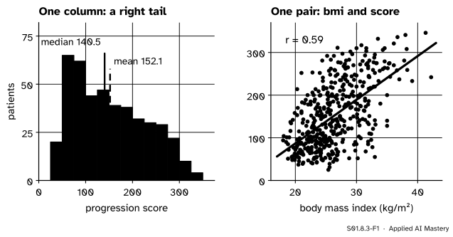
The two views of this lesson. Left: one column, the score, with a long right tail that pulls the mean above the median. Right: one pair, body mass index and the score, the strongest relationship in the table.
The order matters. A correlation between two columns is only as sound as each column on its own: a skewed column, a column with outliers or a column that is a copy of another all change what the correlation means. And a relationship found in all 442 patients may be built from differences between groups rather than from anything that happens inside them, as in S01.7.
Build it up
Step 1. The score alone. It runs from 25 to 346. Its mean is 152.1 and its median 140.5; the quartiles are 87 and 211.5, so the interquartile range is 124.5. The skewness is 0.44: a right tail, as the histogram shows. The fences of S01.4.3 sit at \({87 - 1.5 \times 124.5 = -99.75}\) and \({211.5 + 1.5 \times 124.5 = 398.25}\), so no score is flagged. The score’s shape is mildly skewed, so the report gives the median and quartiles first.
Step 2. The ten measurements alone. The same five numbers for each column, in one table:
Column
Median
IQR
Flagged
age
50
20.75
0
bmi
25.7
6.075
3
bp
93
21
0
s1
186
45.5
8
s2
113
38.45
7
s3
48
17.5
7
s4
4
2
2
s5
4.62
0.721
4
s6
91
14.75
9
“Flagged” counts values beyond the fences. None is impossible, and 40 flags among 3,978 measurements are what tails look like, not errors. The most skewed columns are s3 (0.80), s4 (0.73) and bmi (0.60). sex is a code and gets counts, not a median.
Step 3. Every measurement against the score. One correlation per measurement.
S01.8.3-F4
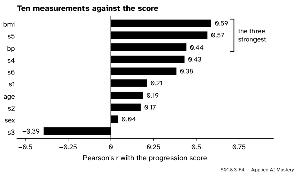
Each measurement’s correlation with the score. Body mass index leads, with s5 close behind; HDL cholesterol (s3) is the only one that falls as the score rises.
Body mass index leads at \({r = 0.59}\), then s5 at 0.57 and blood pressure at 0.44. s3, HDL cholesterol, is negative at \({-0.39}\): higher HDL goes with lower scores. sex is at 0.04, so close to zero that lesson S01.8.4 asks whether it could be chance. Spearman’s rank correlation (S01.5.3) puts s5 first (0.59) and bmi second (0.56): the two leaders are about equally strong, and which one “wins” depends on the measure. That is worth one sentence in the report.
Step 4. Look at the scatter plots behind the numbers. Anscombe’s lesson (S01.5.3): a correlation can hide a curve, a cluster or one far point.
S01.8.3-F5
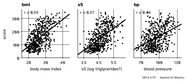
The three strongest pairs. Each is a broad cloud that rises to the right: no curve, no cluster, and no single point that makes the correlation.
None of the three clouds bends, splits or hangs on one point. A straight-line summary is fair for each, and each is loose: a patient’s body mass index leaves most of the score’s spread unexplained.
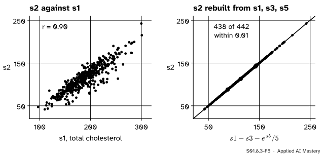
Step 5. Pairs of measurements. Among the 45 pairs of measurements one stands out: s1 (total cholesterol) and s2 (LDL) at \({r = 0.90}\). Two columns that nearly repeat each other should not be reported as two findings, so ask why.
S01.8.3-F6
Why s1 and s2 move together. Right: s2 is, to within 0.01 for 438 of 442 patients, total cholesterol minus HDL minus a fifth of the triglycerides, the Friedewald formula for LDL.
A common way to estimate LDL in the clinic is the Friedewald formula, LDL = total cholesterol − HDL − triglycerides / 5, with every value in mg/dL. If s5 is the natural log of the triglycerides, then \({e^{s5}}\) is the triglycerides, and s1 − s3 − e^s5 / 5 should equal s2. For 438 of the 442 patients it does, to within 0.01. For patient 1,
and s2 is 93.2. So s2 was most likely computed from three other columns, not measured. The check also supports the reading of s5 as a log, and of the cholesterol units as mg/dL. It does not prove them, and the report says “consistent with”.
Step 6. Traps: the leading relationship inside subgroups. Split by the sex code and by three age bands, and recompute the correlation of body mass index with the score in each group.
The formal statement
NoteThe subgroup check
For a relationship between columns \(x\) and \(y\) and a grouping of the rows into groups \(g\) of size \(n_g\), recompute \(r\) inside each group. The relationship holds in every subgroup when each group’s \(r\) has the same sign as the pooled \(r\) and a size of the same order.
Why the check can fail, and how to see that it has not, comes from the sum of products of S01.7.2. Write \({S_{xy} = \sum_i (x_i - \bar{x})(y_i - \bar{y})}\) over all rows, and \(\bar{x}_g\), \(\bar{y}_g\) for the means inside group \(g\). Inside each bracket, add and take away the group mean:
Multiply the two and add over the rows of group \(g\). The two cross terms each contain a sum of deviations from the group’s own mean, which is zero (S01.3.1), so they vanish. What is left, added over the groups, is
The first line is the within-group part: how \(x\) and \(y\) move together inside each group. The second is the between-group part: how the group means line up. Simpson’s reversal in S01.7.2 happened because the between part was large and of the opposite sign. If the within part carries nearly all of \(S_{xy}\), the groups did not make the relationship.
Worked example
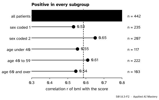
Does the link between body mass index and the score hold in every group?
S01.8.3-F2
The correlation of body mass index with the score, overall (top) and in five subgroups. Every group gives a clearly positive \(r\) between 0.53 and 0.65.
By group. The correlation is 0.53 for the 235 patients coded 1 and 0.65 for the 207 coded 2. In the age bands it is 0.55 under 40 (117 patients), 0.61 from 40 to 59 (222) and 0.54 at 60 and over (103). No group reverses the sign, and none comes close to zero.
By the split of the sum of products, for the sex code. The groups’ means are close to the overall ones. Body mass index averages 26.011 and 26.790 against 26.376 overall, so the groups sit \({-0.365}\) and \({+0.414}\) from it; the score averages 149.021 and 155.667 against 152.133, so they sit \({-3.112}\) and \({+3.534}\) from it. The between part is therefore small:
The within parts are 43,186.5 and 44,332.3, so the pooled sum of products is 88,088.6 (88,089 with unrounded means), and 99.4 percent of it comes from inside the two groups. The relationship is not a by-product of the sex code.
The same check on s5 and blood pressure also gives a positive \(r\) in every group (from 0.43 to 0.61 for s5, from 0.33 to 0.53 for blood pressure). Fifteen correlations computed, none reversed.
Code
From scratch: a correlation function and a loop over the columns.
import numpy as npimport pandas as pdfrom scipy import statsfrom sklearn.datasets import load_diabetestable = load_diabetes(as_frame=True, scaled=False).framey = table["target"].to_numpy()def corr(a, b): a, b = np.asarray(a, dtype=float), np.asarray(b, dtype=float) da, db = a - a.mean(), b - b.mean()returnfloat((da * db).sum() / np.sqrt((da **2).sum() * (db **2).sum()))q1, q3 = np.quantile(y, [0.25, 0.75])print("score: mean", round(y.mean(), 1), " median", np.median(y), " quartiles", q1, q3," skew", round(stats.skew(y), 2))with_score = {name: round(corr(table[name], y), 2) for name in table.columns[:-1]}print(dict(sorted(with_score.items(), key=lambda kv: -kv[1])))
The subgroup check, then the split of the sum of products.
bands = pd.cut(table["age"], [0, 39, 59, 120], labels=["under 40", "40 to 59", "60 and over"])for name, key in (("sex", table["sex"]), ("age band", bands)):print(name, table.groupby(key, observed=True)[["bmi", "target"]].corr().xs("target", level=1)["bmi"].round(2).to_dict())x = table["bmi"]within =sum(((g.bmi - g.bmi.mean()) * (g.target - g.target.mean())).sum() for _, g in table.groupby("sex"))between =sum(len(g) * (g.bmi.mean() - x.mean()) * (g.target.mean() - y.mean()) for _, g in table.groupby("sex"))pooled = ((x - x.mean()) * (y - y.mean())).sum()print("within", round(within), " between", round(between), " pooled", round(pooled)," share within", round(100* within / pooled, 1))
sex {1.0: 0.53, 2.0: 0.65}
age band {'under 40': 0.55, '40 to 59': 0.61, '60 and over': 0.54}
within 87519  between 570  pooled 88089  share within 99.4
The library does the loop in one call: table.corr()["target"] gives every correlation with the score, table.corr(method="spearman") the rank versions, and groupby(...).corr() the subgroup check. The scatter plots are one Axes.scatter call each; the figures above draw them.
Explore
This module’s interactive, the audit trail, lives in lesson S01.8.2. Run its checks with the duplicate and the rent in euros left unfixed, and watch the correlation of area with rent: a relationship is only as sound as the columns under it.
Pitfalls
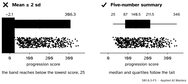
S01.8.3-F3
Wrong beside right. Mean ± 2 standard deviations treats the score as symmetric and runs below zero. The five-number summary follows the data’s own shape.
“Mean ± 2 standard deviations covers the typical range.”
Only for a roughly symmetric column (S01.3.4). For the score it gives \({152.1 \pm 154.2}\), from \({-2.1}\) to 306.3: the lower end is below every score in the table. Report the median and quartiles for a skewed column.
“s1 and s2 both correlate with the score: two findings.”
They are one finding told twice. s2 is computed from s1, s3 and s5, and s1 and s2 have \({r = 0.90}\). In machine learning, a feature built from others adds no new information and can make a linear model’s weights unstable (ML01.9).
“r = 0.59 is strong, so body mass index explains the score.”
A correlation measures how well a straight line fits, not why. Here the cloud is broad, the patients were not assigned their body mass index, and S01.7.3 lists the rival explanations. The report says “goes with”, not “causes”.
Check yourself
Recall
1. In what order does the workflow look at the data, and why that order?
Show answer
One column at a time, then pairs, then pairs inside subgroups. Each step’s conclusions rest on the one before: a correlation is only as sound as the columns, and a pooled relationship may be built from group differences.
2. Which measurement correlates most with the score, and how strongly?
Show answer
Body mass index, \({r = 0.59}\), with s5 close behind at 0.57 (and ahead under Spearman’s rank correlation, 0.59 against 0.56).
3. Why do s1 and s2 correlate at 0.90?
Show answer
s2 (LDL) is, for 438 of 442 patients, s1 − s3 − e^s5 / 5: the Friedewald formula. It was computed from total cholesterol, so it moves with it.
4. What are the two parts of a pooled sum of products?
Show answer
The within-group part, \({\sum_g \sum_{i \in g} (x_i - \bar{x}_g)(y_i - \bar{y}_g)}\), and the between-group part, \({\sum_g n_g (\bar{x}_g - \bar{x})(\bar{y}_g - \bar{y})}\).
5. Which summaries suit the progression score, and why?
Show answer
The median (140.5) and the quartiles (87 and 211.5), because the score is skewed to the right; mean ± 2 standard deviations would run below zero.
Exercises
1.★ The score’s quartiles are 87 and 211.5. Compute the interquartile range and the two fences. The largest score is 346. Is any score flagged?
Show solution
\({\text{IQR} = 211.5 - 87 = 124.5}\), and \({1.5 \times 124.5 = 186.75}\). The fences are
The scores run from 25 to 346, inside both fences, so none is flagged.
2.★★ Patient 2 has s1 = 183, s3 = 70 and s5 = 3.8918, and a stored s2 of 103.2. Check the Friedewald reading of s2.
Show solution
\({e^{3.8918} = 49.00}\), so the triglycerides would be 49 mg/dL and a fifth of them 9.80. Then \({183 - 70 - 9.80 = 103.20}\), which matches the stored 103.2.
3.★★★ Split the same sum of products by the three age bands. The bands have 117, 222 and 103 patients. Their body mass index means sit \({-1.145}\), \({+0.286}\) and \({+0.684}\) from the overall mean, and their score means \({-17.860}\), \({+0.952}\) and \({+18.235}\) from it. The within-group sums of products add up to 84,350.6. Find the between-group part, the pooled sum, and the share that comes from within the bands. Why is the between part larger than for the sex code?
The pooled sum is \({84{,}350.6 + 3{,}737.7 = 88{,}088.3}\), the same total as before up to rounding, since the split changes and the total does not. The share within the bands is \({84{,}350.6 / 88{,}088.3 = 95.8}\) percent. The between part is larger because age lines up with both columns: older bands have a higher mean body mass index and a higher mean score, so the band means rise together. It is still small, and the relationship holds inside every band.
Summary card
One column, then pairs, then pairs inside groups.
S01.8.3-F1
One column, then one pair.
One column. Median and IQR for a skewed column; flags from the fences, judged, not deleted.
Pairs. Rank by \(r\), then look at the scatter plots; explain near-duplicates before reporting them.
Subgroups.\(S_{xy}\) is a within part plus a between part; here 99.4 percent within.
The table’s leaders. bmi 0.59, s5 0.57, bp 0.44; s1 and s2 0.90, because s2 is computed.
Sources and next steps
Sources. Each was opened and checked against this lesson on 12 November 2026.
MSD Manual, Friedewald equation for low-density lipoprotein: LDL = total cholesterol − triglycerides / 5 − HDL, not valid for triglycerides of 400 mg/dL or more, citing Friedewald, Levy and Fredrickson, Clinical Chemistry 18 (1972), 499 to 502.