\( \newcommand{\vect}[1]{\mathbf{#1}} \newcommand{\mat}[1]{\mathbf{#1}} \newcommand{\R}{\mathbb{R}} \newcommand{\E}{\mathbb{E}} \newcommand{\Prob}{\mathbb{P}} \newcommand{\T}{^{\top}} \newcommand{\norm}[1]{\lVert #1 \rVert} \newcommand{\abs}[1]{\lvert #1 \rvert} \newcommand{\ihat}{\mkern1mu\hat{\boldsymbol{\imath}}\mkern2mu} \newcommand{\jhat}{\mkern1mu\hat{\boldsymbol{\jmath}}\mkern2mu} \newcommand{\pd}[2]{\frac{\partial #1}{\partial #2}} \newcommand{\argmax}{\operatorname*{arg\,max}} \newcommand{\argmin}{\operatorname*{arg\,min}} \newcommand{\cdata}[1]{\class{c-data}{#1}} \newcommand{\cmodel}[1]{\class{c-model}{#1}} \newcommand{\ctruth}[1]{\class{c-truth}{#1}} \newcommand{\cgrad}[1]{\class{c-grad}{#1}} \newcommand{\closs}[1]{\class{c-loss}{#1}} \newcommand{\cparam}[1]{\class{c-param}{#1}} \newcommand{\csecond}[1]{\class{c-second}{#1}} \renewcommand{\,}{\mkern3mu} \)

Histograms and the choice of bins

A histogram counts values into bins and draws a bar for each. Build one by hand for nine rents, see how the bin width and the starting point change the picture, and learn why densities, not counts, are the honest heights.

S01.4.1L1 Core25 minIn review

Before this lesson

S01.3 Center, spread and shape P02.8 Plotting with Matplotlib and seaborn (planned)

After this lesson you can

• Draw a histogram of a small data set by hand, stating the bin width, the starting point and which bin a value on an edge belongs to.
• Show with an example that the shape of a histogram changes with both the bin width and the starting point.
• Turn counts into proportions and densities, and explain why only densities make bins of unequal width comparable.
• Compute the square-root, Sturges and Freedman-Diaconis bin widths, and bin data with a loop and with numpy.histogram.

In review. The maths and code on this page are checked by automated tests on every change, but an independent reader has not signed it off yet. Spot a mistake or a confusing step? Tell us.

The question

Two analysts draw a histogram of the same nine rents. One sees a single peak with a long tail to the right. The other sees two equal bars and a lonely one far away. Neither has made a mistake. How can one list of numbers give two different pictures, and which picture should you believe before you feed that column to a model?

Intuition

The nine rents are the rent column of the course’s invented flats table, in hundreds of euros a month: 3, 4, 7, 7, 8, 9, 10, 12 and 30. The 30 is the penthouse.

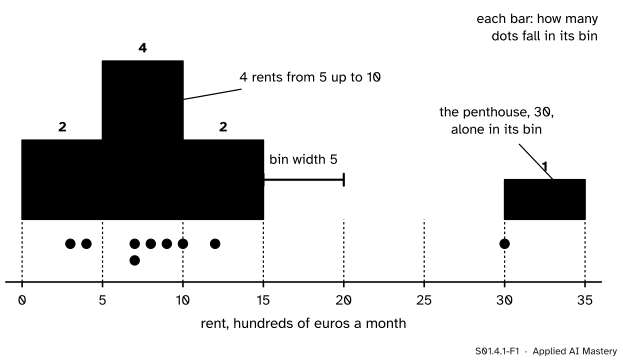
A dot plot (S01.3) puts each value on a number line. A histogram goes one step further. It cuts the number line into intervals of equal length, called bins, counts how many values fall into each bin, and draws a bar as tall as that count.

S01.4.1-F1

The nine rents counted into bins of width 5. Each bar stands over its bin and is as tall as the number of dots underneath it.

The bars are the dots, piled up. Where many values sit close together, a tall bar stands; where there are none, the line stays bare. That is the whole idea, and it is why a histogram shows the shape of a column at a glance: where it is crowded, where it thins out, and where a value sits far from the rest.

But look at what had to be decided first. Someone chose that the bins are 5 wide and that the first one starts at 0. The data did not choose these. Change either and the bars change.

Build it up

Step 1. The bins. Choose a starting point \(a\) and a width \(h\). The bin edges are then \(a,\ a + h,\ a + 2h, \dots\) For the anchor picture, \(a = 0\) and \(h = 5\), so the edges are 0, 5, 10, 15, 20, 25, 30, 35.

Step 2. Who owns an edge. A rent of exactly 10 sits on the edge between two bins. A rule must decide, and the usual one (NumPy’s) is that a bin includes its left edge and excludes its right edge: the bin from 5 to 10 is written \([5, 10)\) and holds values \(x\) with \({5 \le x < 10}\). So 10 belongs to \([10, 15)\). NumPy closes the very last bin on both sides, so that the largest value is never lost.

Step 3. Count. Go through the nine rents once and add one to the count of the bin each falls into. With \(a = 0\) and \(h = 5\) the counts are 2, 4, 2, 0, 0, 0, 1.

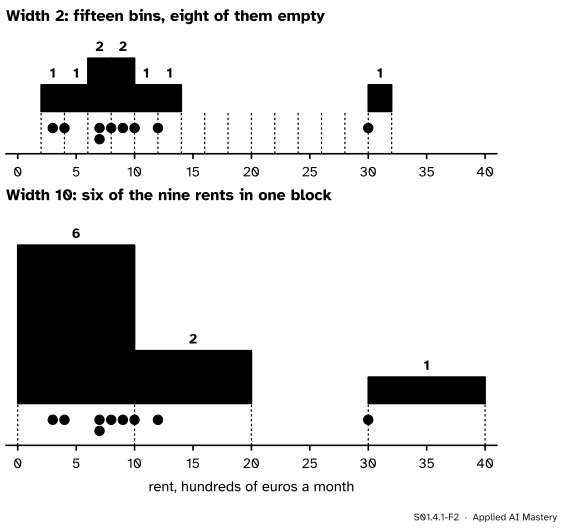
Step 4. Change the width. Now try a narrow width and a wide one.

S01.4.1-F2

The same nine rents with bins too narrow and too wide. Width 2 turns the histogram back into a dot plot with gaps. Width 10 puts six rents into one block and hides the difference between 3 and 9.

With width 2 almost every bar holds one or two rents, and the picture is mostly noise: the gaps between bars say more about where the edges fell than about rents. With width 10 the cheap and the middle flats are lumped together. There is no right width written in the data; a good width is wide enough to smooth out the accidents of a small sample and narrow enough to keep real features.

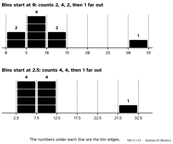
Step 5. Change the start. Keep the width at 5 but start the bins at 2.5 instead of 0. The worked example below does this by hand, and the peak at 5 to 10 disappears.

Step 6. Choose what a bar’s height means. So far a height is a count. Dividing by the number of values \(n\) gives a proportion, the share of the data in that bin. Dividing the proportion by the bin width gives a density. The next section shows why the third is the one that keeps its meaning when bins differ in width.

The formal statement

NoteDefinition: histogram

Take \(n\) values and bin edges \({b_0 < b_1 < \dots < b_k}\). Bin \(j\) is the interval \([b_{j-1}, b_j)\) (the last bin also includes \(b_k\)), with width \({h_j = b_j - b_{j-1}}\). Let \(n_j\) be the number of values in bin \(j\). Its bar can be drawn with three heights:

• count \(n_j\);
• proportion \({p_j = n_j / n}\);
• density \({d_j = p_j / h_j}\).

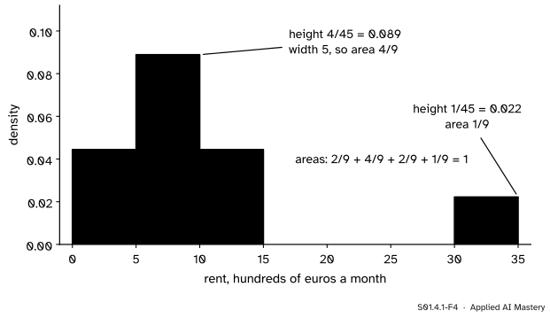
The areas of a density histogram add up to 1. The area of bar \(j\) is its height times its width, and the widths cancel:

\[ d_j \, h_j \;=\; \frac{p_j}{h_j}\, h_j \;=\; p_j . \]

Every value lies in exactly one bin, so the counts add up to \(n\). Adding the areas over all bins,

\[ \begin{aligned} \sum_{j=1}^{k} d_j h_j &= \sum_{j=1}^{k} p_j = \sum_{j=1}^{k} \frac{n_j}{n} \\ &= \frac{1}{n} \sum_{j=1}^{k} n_j = \frac{n}{n} = 1 . \end{aligned} \]

So on the density scale the area of a bar is the share of the data in its bin, whatever the bin’s width. That is why densities are the only heights that let bins of unequal width be compared, and why this scale becomes the probability density of M06.6.1, where the area under a curve is a probability.

S01.4.1-F4

The anchor histogram on the density scale. Height times width is each bin’s share of the rents, and the shares add to 1.

Rules for the width. Three rules are built into NumPy. For \(n\) values whose range (largest minus smallest) is \(R\):

• square root: use \({k = \lceil \sqrt{n}\, \rceil}\) bins, of width \(R / k\);
• Sturges: use \({k = \lceil \log_2 n \rceil + 1}\) bins, of width \(R / k\);
• Freedman-Diaconis: take the width

\[ h \;=\; \frac{2\,\mathrm{IQR}}{n^{1/3}} . \]

The first two look only at how many values there are. The Freedman-Diaconis rule also looks at their spread, measured by the interquartile range of S01.3.2, which one extreme value cannot pull far: with or without the penthouse, the IQR of the rents is 3. Its \(n^{1/3}\) means the bins narrow slowly as the data grow: eight times as many values with the same IQR give bins half as wide. NumPy turns a width \(h\) into a whole number of bins, \({\lceil R / h \rceil}\), and then spreads them evenly over the range, so the width it uses can be a little smaller than \(h\).

Worked example

Bin the nine rents with width 5, first starting at 0, then starting at 2.5.

Starting at 0. The edges are 0, 5, 10, …, 35. Take the rents in order. 3 and 4 fall into \([0, 5)\). 7, 7, 8 and 9 fall into \([5, 10)\). 10 falls into \([10, 15)\), because a bin keeps its left edge, and so does 12. The bins from 15 to 30 stay empty. 30 falls into \([30, 35)\). The counts are 2, 4, 2, 0, 0, 0, 1, which add to 9.

Starting at 2.5. The edges are 2.5, 7.5, 12.5, …, 32.5. Now 3, 4, 7 and 7 share \([2.5, 7.5)\), and 8, 9, 10 and 12 share \([7.5, 12.5)\). The penthouse is alone in \([27.5, 32.5)\). The counts are 4, 4, 0, 0, 0, 1.

S01.4.1-F3

The worked example as a tally. Same rents, same width: starting the bins half a width later turns a peak into two equal bars.

Both histograms are correct. They answer slightly different questions, because the edges decide which rents are counted as neighbours. 7 and 8 sit in different bins in the first picture and in the same bin in the second.

Densities for the first version. The bin \([5, 10)\) holds 4 of the 9 rents, a proportion \({4/9 = 0.444}\). Its density is that proportion over the width: \({0.444 / 5 = 4/45 = 0.0889}\) per hundred euros. The lone bin of the penthouse has density \({(1/9)/5 = 1/45 = 0.0222}\).

The rules for these rents. With \(n = 9\) and range \({R = 30 - 3 = 27}\):

• square root: \({\lceil \sqrt{9}\, \rceil = 3}\) bins of width \({27/3 = 9}\);
• Sturges: \({\log_2 9 = 3.17}\), so \({\lceil 3.17 \rceil + 1 = 5}\) bins of width \({27/5 = 5.4}\);
• Freedman-Diaconis: the IQR is \({10 - 7 = 3}\) and \({9^{1/3} = 2.080}\), so

\[ h = \frac{2 \times 3}{2.080} = 2.88 . \]

NumPy then uses \({\lceil 27 / 2.88 \rceil = \lceil 9.36 \rceil = 10}\) bins of width 2.7. Three rules, three answers from 2.7 to 9: the rules are starting points, not verdicts.

Code

First from scratch: a loop that finds each value’s bin. The bin of \(x\) is the whole number of widths it lies past the start, \({\lfloor (x - a)/h \rfloor}\).

import math

rents = [3, 4, 7, 7, 8, 9, 10, 12, 30]

def histogram(values, start, width):
    """Counts in bins [start + k*width, start + (k+1)*width), enough bins to hold the largest value."""
    k = math.floor((max(values) - start) / width) + 1
    counts = [0] * k
    for x in values:
        counts[math.floor((x - start) / width)] += 1
    return counts

from_0 = histogram(rents, 0, 5)
from_2_5 = histogram(rents, 2.5, 5)
print("width 5 from 0:  ", from_0)
print("width 5 from 2.5:", from_2_5)
print("width 2 from 2:  ", histogram(rents, 2, 2))
print("width 10 from 0: ", histogram(rents, 0, 10))

n = len(rents)
density = [c / n / 5 for c in from_0]
print("densities:", [round(d, 4) for d in density], " total area:", round(sum(d * 5 for d in density), 10))

width 5 from 0:   [2, 4, 2, 0, 0, 0, 1]
width 5 from 2.5: [4, 4, 0, 0, 0, 1]
width 2 from 2:   [1, 1, 2, 2, 1, 1, 0, 0, 0, 0, 0, 0, 0, 0, 1]
width 10 from 0:  [6, 2, 0, 1]
densities: [0.0444, 0.0889, 0.0444, 0.0, 0.0, 0.0, 0.0222]  total area: 1.0

Now NumPy. numpy.histogram takes the edges, or a number of bins, or the name of a rule, and returns the counts with the edges it used; density=True returns densities instead.

import numpy as np

r = np.array(rents, dtype=float)
counts, edges = np.histogram(r, bins=np.arange(0, 36, 5))
dens, _ = np.histogram(r, bins=np.arange(0, 36, 5), density=True)
print("counts:", counts, " densities:", dens.round(4))

q1, q3 = np.quantile(r, [0.25, 0.75])
fd = 2 * (q3 - q1) / len(r) ** (1 / 3)
print(f"Freedman-Diaconis width by hand: {fd:.2f}")
for rule in ["sqrt", "sturges", "fd"]:
    e = np.histogram_bin_edges(r, bins=rule)
    print(f"{rule:8s} {len(e) - 1:2d} bins of width {e[1] - e[0]:.2f}")

counts: [2 4 2 0 0 0 1]  densities: [0.0444 0.0889 0.0444 0.     0.     0.     0.0222]
Freedman-Diaconis width by hand: 2.88
sqrt      3 bins of width 9.00
sturges   5 bins of width 5.40
fd       10 bins of width 2.70

The same rule on real data. The explorer below uses the petal lengths of every fourth flower in scikit-learn’s iris data, 38 values that ship with the library.

from sklearn.datasets import load_iris

petals = load_iris().data[::4, 2]              # petal length in cm, flowers 0, 4, 8, ..., 148
p1, p3 = np.quantile(petals, [0.25, 0.75])
fd_iris = 2 * (p3 - p1) / len(petals) ** (1 / 3)
c_fd, e_fd = np.histogram(petals, bins="fd")
print(f"{len(petals)} petals, IQR {p3 - p1:.3f}, Freedman-Diaconis width {fd_iris:.2f}")
print("fd bins:", e_fd.round(2), "counts:", c_fd)
print("width 0.5 from 1:", np.histogram(petals, bins=np.arange(1.0, 6.51, 0.5))[0])

38 petals, IQR 4.025, Freedman-Diaconis width 2.39
fd bins: [1.3  3.65 6.  ] counts: [15 23]
width 0.5 from 1: [ 8  5  0  0  0  3  3  6  1 11  1]

To draw any of these, Axes.hist(values, bins=...) in Matplotlib does the counting and the drawing in one call (P02.8.2); its density=True gives the density scale.

Explore

S01.4-X1

Histogram bin-width explorer

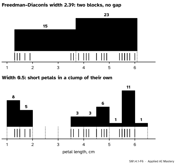
Slide the bin width from wide to narrow and watch the two clumps of petals merge into one block, separate, and then shatter into single flowers. Then keep the width fixed and slide where the first bin starts: at some widths the gap between the clumps opens and closes as the edges move.

Notice that the Freedman-Diaconis width, 2.39 here, gives only two bars and hides the gap between 1.9 and 3.5 cm. The data have two clumps, so their IQR runs from one clump into the other and is large, and the rule picks wide bins. A rule is a first guess; the reader’s eye is the check.

Pitfalls

S01.4.1-F5

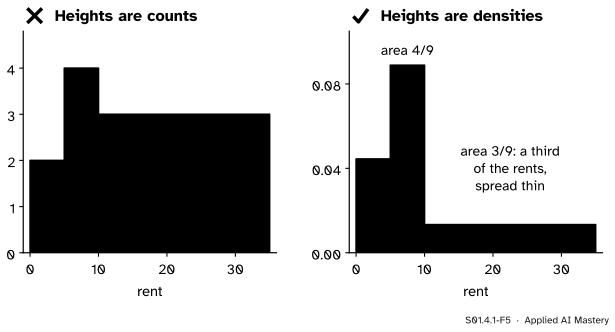
Wrong beside right. With unequal bins, count heights make the wide bin look like the largest group. Density heights make each bar’s area its share.

“Bins of different widths are fine if I label the counts.”

The eye reads area, not height. On the left above, three rents spread over 25 units draw a block larger than the other two bars together. Use densities, so that area means share. Equal-width bins avoid the question, which is why they are the default.

“The histogram shows the shape of the data.”

It shows the data seen through one choice of width and start. The worked example turned a peak into two equal bars by moving the edges half a width. Before you describe a shape, try two or three widths and two starts, and trust only the features that survive all of them. This matters when a histogram decides a modelling step, such as taking logs of a skewed feature.

“A bin rule gives the right answer.”

The three rules gave 3, 5 and 10 bins for the same nine rents. NumPy’s own notes call Sturges’ rule too conservative for large data that are not bell-shaped, and the Freedman-Diaconis rule hid the two clumps of the iris petals. Rules are a starting point for your own look.

“A value on an edge goes in both bins, or either.”

It goes in exactly one, by a fixed rule. NumPy keeps the left edge and drops the right, except for the last bin. If two tools disagree, check this rule before you check the data.

Check yourself

Recall

1. Which two choices must be made before a histogram can be drawn?

Show answer

The bin width and where the first bin starts. Together they fix every bin edge.

2. With bins of width 5 starting at 0, which bin holds the rent 10, and why?

Show answer

The bin from 10 to 15, because each bin includes its left edge and excludes its right edge.

3. How is a density height computed, and what does the area of a density bar mean?

Show answer

Density is the proportion in the bin divided by the bin width, \({d_j = (n_j/n)/h_j}\). The area, height times width, is the proportion of the data in that bin, so the areas add to 1.

4. State the Freedman-Diaconis width and its value for the nine rents.

Show answer

\(h = 2\,\mathrm{IQR}/n^{1/3}\). For the rents the IQR is 3 and \(n = 9\), so \({h = 6 / 2.080 = 2.88}\).

5. Why do bins of unequal width need density heights?

Show answer

Because a reader judges a bar by its area. With count heights a wide bin draws a large area from a few values. With density heights each bar’s area is its share of the data.

Exercises

1. ★ Bin the nine rents with width 4 starting at 2. Give the counts and the density of the tallest bar.

Show solution

The edges are 2, 6, 10, …, 34. The bin \([2, 6)\) holds 3 and 4; \([6, 10)\) holds 7, 7, 8 and 9; \([10, 14)\) holds 10 and 12; the four bins from 14 to 30 are empty; \([30, 34)\) holds 30. The counts are 2, 4, 2, 0, 0, 0, 0, 1. The tallest bar has density \({(4/9)/4 = 1/9 = 0.111}\).

2. ★★ A column has \(n = 64\) values, range 40 and IQR 8. How many bins, and of what width, does each of the three rules give?

Show solution

Square root: \({\lceil \sqrt{64}\, \rceil = 8}\) bins of width \({40/8 = 5}\). Sturges: \({\log_2 64 = 6}\), so \({6 + 1 = 7}\) bins of width \({40/7 = 5.71}\). Freedman-Diaconis: \({64^{1/3} = 4}\), so \({h = 2 \times 8 / 4 = 4}\), and \({40/4 = 10}\) bins of width 4 exactly.

3. ★★★ Two neighbouring bins have the same width \(h\) and densities \(d_1\) and \(d_2\). They are merged into one bin of width \(2h\). Show that the merged bar’s density is the average \({(d_1 + d_2)/2}\), and check it on the anchor histogram by merging \([10, 15)\) with \([15, 20)\).

Show solution

The proportions of the two bins are their areas, \({d_1 h}\) and \({d_2 h}\). The merged bin holds both groups of values, so its proportion is \({d_1 h + d_2 h}\). Its density is that proportion over its width:

\[ \begin{aligned} \frac{d_1 h + d_2 h}{2h} &= \frac{(d_1 + d_2)\,h}{2h} \\ &= \frac{d_1 + d_2}{2} . \end{aligned} \]

For the rents, \([10, 15)\) has density \({2/45}\) and \([15, 20)\) has 0. The merged bin \([10, 20)\) holds 2 of 9 rents over a width of 10, density \({(2/9)/10 = 1/45}\), which is the average of \({2/45}\) and 0.

Summary card

A histogram is the data counted into bins that you chose.

S01.4.1-F1

Bars count the dots in each bin.

• Bins. Edges \(a, a + h, a + 2h, \dots\); each bin keeps its left edge.
• Heights. Count \(n_j\), proportion \(n_j/n\), density \({(n_j/n)/h_j}\); density areas add to 1.
• Width rules. \(\lceil\sqrt{n}\,\rceil\) bins; \({\lceil \log_2 n \rceil + 1}\) bins; \({h = 2\,\mathrm{IQR}/n^{1/3}}\).
• Habit. Try several widths and starts; trust features that survive.

Sources and next steps

Sources. Each was opened and checked against this lesson on 12 November 2026.

• NIST/SEMATECH, e-Handbook of Statistical Methods, section 1.3.3.14, Histogram. Equal-sized bins called classes, the relative histogram whose heights are normalised to sum to one, and the version divided by the class width, whose area is one.
• NumPy, numpy.histogram. All bins but the last are half-open, the last includes its right edge, and density=True makes the integral over the range 1.
• NumPy, numpy.histogram_bin_edges. The ‘sqrt’, ‘sturges’ and ‘fd’ rules with their formulas, the final bin count taken as the ceiling of range over width, and the note that Sturges is too conservative for large non-normal data.
• David Diez, Mine Cetinkaya-Rundel and Christopher Barr, OpenIntro Statistics, 4th edition (free PDF). Section 2.1, Examining numerical data, covers histograms and box plots at this level.
• scikit-learn, load_iris: 150 flowers, 50 of each of three species, four measurements each.

Next. S01.4.2 The cumulative view draws the same data with no bins at all.

This lesson unlocks

S01.4.2 The cumulative view: ECDF and quantiles M06.6 Continuous random variables and densities (planned)

Your progress is saved in this browser only. No account, no tracking.