A table is a sample from something larger. Name the target population, the sampling frame and the sample, tell a parameter from a statistic, and see why a simple random sample has means that average out to the population mean.
Name the target population, the sampling frame and the sample behind a data set, and say which units could never have been drawn.
Tell a parameter from a statistic, writing the population mean as mu and the sample mean as x-bar.
State what makes a sample simple random: every set of n units has the same chance of being the sample.
List every sample of two from a small population and show that their means average exactly to the population mean.
Draw a simple random sample in Python, first by shuffling from scratch and then with NumPy and pandas.
In review. The maths and code on this page are checked by automated tests on every change, but an independent reader has not signed it off yet. Spot a mistake or a confusing step? Tell us.
The question
The flats table holds nine flats, and their mean rent is 10 (hundreds of euros a month). Does that tell you the typical rent of a flat in the city? It depends on one thing the table does not show: how those nine flats got into it. Every model in machine learning faces the same question about its training rows.
Intuition
The flats table of module S01.1 was never the point in itself. Nobody cares about nine particular flats. We care about the flats of the city, and the nine are a window onto them. This lesson names the parts of that window.
S01.2.1-F1
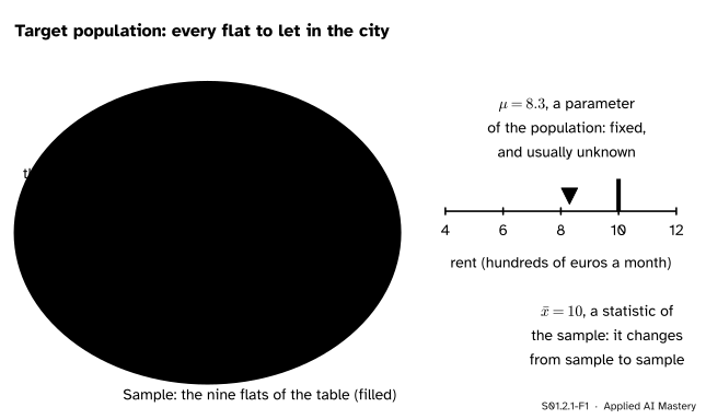
Three layers. The target population is what the question is about, the sampling frame is the list the sample was drawn from, and the sample is what ended up in the table. On the right, the population’s mean is a fixed number; the sample’s mean is one draw of a number that changes with the sample.
Read the picture from the outside in.
The target population is every unit the question is about: here every flat to let in the city. It is fixed by the question, not by the data.
The sampling frame is the list you can actually draw from: here the listings of one website. A flat that is not on the website can never reach the table, however carefully the draw is made.
The sample is the units that were drawn: here the nine flats of the table.
A number that describes the whole population is a parameter. The population mean rent is written \(\ctruth{\mu}\) (Greek mu). It is one fixed number, and in real life it is usually unknown, because nobody has measured every flat. A number computed from the sample is a statistic. The sample mean is written \(\cmodel{\bar{x}}\) (x-bar). It is known as soon as you have the table, but draw a different sample and it changes.
For the course we built an invented city of 500 flats, so we know its mean: \(\ctruth{\mu} = 8.3\). The nine flats give \(\cmodel{\bar{x}} = 10\). From here on the course keeps the two kinds of letter apart: Greek letters for a population, Latin letters for a sample.
Build it up
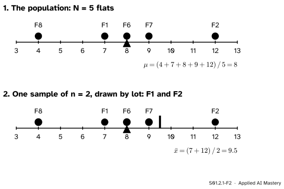
The city is too big to work with by hand, so we shrink it. Take a population of just five flats, five of the nine from the table, with rents 4, 7, 8, 9 and 12. We write \(N = 5\) for the size of a population and \(n\) for the size of a sample.
Step 1. The parameter. With all five flats in front of us, the population mean is a plain average: the rents add to 40, so \(\ctruth{\mu} = 40 / 5 = 8\).
Step 2. One sample. Write the five names on slips, mix them in a hat and draw two. Suppose F1 and F2 come out, with rents 7 and 12. The sample mean is \(\cmodel{\bar{x}} = 19 / 2 = 9.5\), which misses \(\ctruth{\mu}\) by 1.5.
S01.2.1-F2
The population mean stays at 8 (triangle). The mean of one sample of two, F1 and F2, is 9.5 (bar).
Step 3. Another draw, another answer. Put the slips back and draw again: perhaps F8 and F6, with mean 6. The statistic moved; the parameter did not. That is the whole difference between them.
Step 4. How many samples are there? A sample of two is a set of two flats, in no order, so the number of possible samples is the number of ways to choose 2 from 5, which lesson M01.8.3 counts:
\[
\binom{5}{2} = \frac{5 \times 4}{2} = 10.
\]
Drawing slips from a well-mixed hat makes each of these ten sets equally likely, with chance \(1/10\) each. That property has a name.
The formal statement
NoteDefinitions
A population is a set of \(N\) units with values \(x_1, \dots, x_N\). Its mean is the parameter
A sample is a set of \(n\) of those units. Its mean is the statistic \(\cmodel{\bar{x}}\): the sum of the \(n\) sampled values divided by \(n\).
A sample is a simple random sample of size \(n\) when every set of \(n\) units has the same chance of being the sample. There are \(\binom{N}{n}\) such sets, so each has chance \(1 / \binom{N}{n}\).
In a simple random sample a unit is drawn at most once: the five slips do not go back into the hat until the sample is complete. Drawing without replacement is the default meaning of “simple random sample” in this course.
Consequence 1: every unit has the same chance, \(n/N\). Fix one unit, say F2. A sample that contains F2 is F2 plus \(n - 1\) of the other \(N - 1\) units, so \(\binom{N-1}{n-1}\) samples contain it. Its chance of being drawn is the share of samples that contain it:
The first two lines write both counts out in factorials, the third cancels \({(N - n)!}\), and the last uses \(N! = N \cdot {(N-1)!}\) and \(n! = n \cdot {(n-1)!}\). For the five flats and \(n = 2\): \(\binom{4}{1} = 4\) samples contain each flat, out of 10, a chance of \(4/10 = 2/5\).
Consequence 2: the sample means average exactly to \(\ctruth{\mu}\). List all \(\binom{N}{n}\) samples and add up their means. Each mean is a sum over its sample divided by \(n\), so the total is
In the double sum each unit’s value is counted once for every sample that contains it, which is \(\binom{N-1}{n-1}\) times (Consequence 1). So the double sum equals \(\binom{N-1}{n-1}\) times the population total. Dividing the total of the means by the number of samples gives their average:
No single sample has to hit \(\ctruth{\mu}\). But taken over every sample the draw could produce, the sample mean is centred exactly on it. A method of choosing that has this property cannot lean one way: the next lesson calls it having no bias.
Go deeper: what changes if the slips go back into the hat
Drawing with replacement puts each slip back before the next draw, so a flat can appear twice. Then the \(N^n\) ordered draws are equally likely: 25 of them for two draws from five flats. Each flat appears as the first draw in 5 of them and as the second draw in 5 of them, so the total of the 25 means is \(\tfrac{1}{2}{({5 \cdot 40} + {5 \cdot 40})} = 200\), and their average is \(200 / 25 = 8\) again. The centre is still \(\ctruth{\mu}\). What changes is the spread of the means, which lesson S01.3.3 measures, and which matters when the sample is a large part of a small population. Sampling with replacement is also the setting of the bootstrap (S02.8).
Worked example
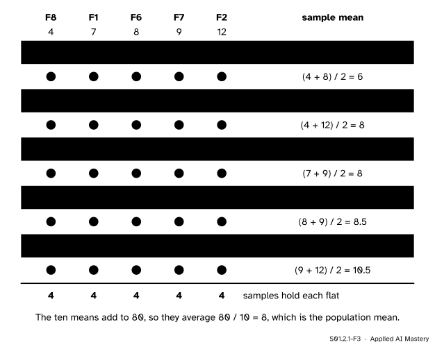
All samples of two from the five flats. The ten sets, with their means, are traced below.
S01.2.1-F3
The ten samples of two. Each column has four filled circles, so each flat is in four samples, and the ten means add to 80.
Their average is \(80 / 10 = 8\), which is \(\ctruth{\mu}\), as Consequence 2 promised. The shortcut gives the same total without the list: each flat is in 4 samples, so the ten sample sums add to \({4 \times 40} = 160\), and halving each sum to make a mean gives 80.
S01.2.1-F4
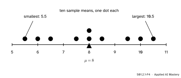
The ten sample means as dots. They run from 5.5 to 10.5 and balance on \(\ctruth{\mu} = 8\), yet only two of the ten land on it.
Two things show in the dot plot. The means are spread out: a sample of two can miss by as much as 2.5 either way. And they are spread evenly about 8, with nothing pulling them to one side. The next lesson gives each of those two things a number.
Code
First a simple random sample from scratch. Shuffle the units, then keep the first \(n\). The shuffle walks from the last position to the first and swaps each item with one at a random position at or before it (the Fisher-Yates shuffle), which makes every order of the units equally likely.
import itertoolsimport numpy as npids = ["F8", "F1", "F6", "F7", "F2"]rent = {"F8": 4, "F1": 7, "F6": 8, "F7": 9, "F2": 12}def shuffle(items, rng): items =list(items)for i inrange(len(items) -1, 0, -1): j =int(rng.integers(0, i +1)) # a position from 0 to i items[i], items[j] = items[j], items[i]return itemsdef simple_random_sample(units, n, rng):return shuffle(units, rng)[:n]rng = np.random.default_rng(2026)counts = {}for _ inrange(10_000): pair =frozenset(simple_random_sample(ids, 2, rng)) counts[pair] = counts.get(pair, 0) +1print("different samples seen:", len(counts))print("smallest and largest count:", min(counts.values()), max(counts.values()))
different samples seen: 10
smallest and largest count: 935 1040
In 10,000 draws all ten samples turn up, each close to 1,000 times. Now list them exactly, as in the worked example, and check both consequences.
samples =list(itertools.combinations(ids, 2))means = [(rent[a] + rent[b]) /2for a, b in samples]mu =sum(rent.values()) /len(rent)print("number of samples:", len(samples))print("means:", sorted(means))print("average of the means:", sum(means) /len(means), " mu:", mu)print("samples holding each flat:", [sum(f in s for s in samples) for f in ids])
number of samples: 10
means: [5.5, 6.0, 6.5, 7.5, 8.0, 8.0, 8.5, 9.5, 10.0, 10.5]
average of the means: 8.0  mu: 8.0
samples holding each flat: [4, 4, 4, 4, 4]
The library calls do the shuffle for you. NumPy’s Generator.choice must be told replace=False, because its default draws with replacement. pandas’ DataFrame.sample draws without replacement by default and takes a seed as random_state.
import pandas as pdrng = np.random.default_rng(7)print("numpy:", rng.choice(ids, size=2, replace=False))flats = pd.DataFrame({"id": ids, "rent": [rent[f] for f in ids]})draw = flats.sample(n=2, random_state=7)print(draw)print("sample mean:", draw["rent"].mean())
Which two flats a seed gives is not worth remembering, and a new version of a library may give others. What matters is that the same seed gives the same sample every time the script runs on the same versions, so a result can be checked (P02.9).
Explore
This module’s interactive, the sampling bench, lives in the next lesson. There you draw sample after sample from a population of 48 flats and watch where the sample means land.
Pitfalls
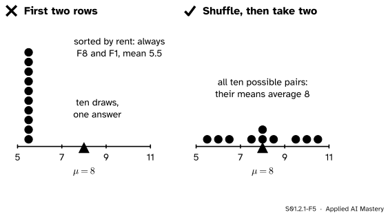
S01.2.1-F5
Wrong beside right. Taking the first rows of a list sorted by rent gives the same sample every time, far below \(\ctruth{\mu}\). Shuffling first gives every pair a chance, and the means centre on 8.
“The first rows of the file are as good as any other rows.”
Only if the file is in random order, and files rarely are. They are sorted by date, by price, by postcode or by whoever entered them. Taking the head of a list sorted by rent gives F8 and F1 every time, a mean of 5.5. The same mistake in machine learning is to split a file into training and test rows without shuffling it first.
“rng.choice(units, size=n) draws a simple random sample.”
Its default is replace=True, so a unit can be drawn twice and the sample can hold fewer than \(n\) different units. Pass replace=False. DataFrame.sample has the opposite default.
“Every flat has the same chance of being picked, so the sample is simple random.”
Equal chances for each unit are not enough. Seat the five flats round a table and pick one pair of neighbours at random: F8 and F1, F1 and F6, F6 and F7, F7 and F2, or F2 and F8. Every flat is in two of the five pairs, so each has chance \(2/5\), exactly as before. But F8 and F6 can never be drawn together, so not every set of two has the same chance. Simple random means equal chances for every set of \(n\) units.
Check yourself
Recall
1. What are the target population, the sampling frame and the sample for the flats table?
Show answer
The target population is every flat to let in the city, the sampling frame is the listings of one website, and the sample is the nine flats of the table.
2. Which of these is a parameter and which a statistic: the mean rent of the city’s 500 flats, and the mean rent of the nine flats?
Show answer
The city’s mean, \(\mu = 8.3\), is a parameter: fixed, and usually unknown. The nine flats’ mean, \(\bar{x} = 10\), is a statistic: it changes from sample to sample.
3. What makes a sample of size \(n\) a simple random sample?
Show answer
Every set of \(n\) units of the population has the same chance of being the sample.
4. In a simple random sample of \(n\) from \(N\), what is the chance that one given unit is drawn?
Show answer
\(n / N\), because \(\binom{N-1}{n-1}\) of the \(\binom{N}{n}\) samples contain it, and that ratio is \(n / N\).
5. The ten samples of two from the rents 4, 7, 8, 9, 12 have means from 5.5 to 10.5. What do they average, and why?
Show answer
Exactly 8, the population mean. Each flat is in four of the ten samples, so every rent counts equally in the total of the means.
Exercises
1.★ A population of four flats has rents 3, 7, 9 and 13. List every simple random sample of two with its mean, and check that the means average to \(\mu\).
Show solution
\(\mu = 32 / 4 = 8\). There are \(\binom{4}{2} = 6\) samples: \(\{3, 7\}\) mean 5, \(\{3, 9\}\) mean 6, \(\{3, 13\}\) mean 8, \(\{7, 9\}\) mean 8, \(\{7, 13\}\) mean 10 and \(\{9, 13\}\) mean 11. The means add to 48, and \(48 / 6 = 8 = \mu\).
2.★★ From the five flats (rents 4, 7, 8, 9, 12) we now draw simple random samples of three. How many samples are there, how many contain F2, and what do the sample means average? Answer without listing the samples.
Show solution
There are \(\binom{5}{3} = 10\) samples. Those that contain F2 add two of the other four flats, so there are \(\binom{4}{2} = 6\) of them, a chance of \(6/10 = 3/5 = n/N\). Each flat is in 6 samples, so the ten sample sums add to \({6 \times 40} = 240\). Each mean is a sum divided by 3, so the means add to 80 and average \(80 / 10 = 8 = \mu\).
3.★★★ In the round-table scheme of the third pitfall, list the five possible samples with their means. Show that the means average to \(\mu = 8\) and name the five sets of two that can never be drawn. Is this scheme a simple random sample?
Show solution
The pairs are F8 and F1, mean \({(4 + 7)/2} = 5.5\); F1 and F6, mean 7.5; F6 and F7, mean 8.5; F7 and F2, mean 10.5; F2 and F8, mean 8. The means add to 40, and \(40 / 5 = 8\), because each flat is in exactly two pairs. The sets that can never be drawn are F8 and F6, F8 and F7, F1 and F7, F1 and F2, and F6 and F2. Half of the ten sets have chance 0 and the other half chance \(1/5\), so this is not a simple random sample, even though each flat has chance \(2/5\) and the means are centred on \(\mu\).
Summary card
A table is a sample: say from what, and how it was drawn.
S01.2.1-F1
Population, frame, sample; parameter, statistic.
Parameter\(\mu\), of the population: fixed, usually unknown. Statistic\(\bar{x}\), of the sample: it varies.
Simple random sample: each of the \(\binom{N}{n}\) sets of \(n\) units has chance \(1 / \binom{N}{n}\).
Each unit is drawn with chance \(n / N\).
Over all samples the mean of \(\bar{x}\) is exactly \(\mu\).
Sources and next steps
Sources. Each was opened and checked against this lesson on 12 November 2026.
David Diez, Mine Cetinkaya-Rundel and Christopher Barr, OpenIntro Statistics, 4th edition (free PDF). Section 1.3.1 defines the target population and the sample, and Section 1.3.3 describes a simple random sample as a raffle and warns that a sample picked by hand can be biased without meaning to be.
Barbara Illowsky and Susan Dean, Introductory Statistics 2e, OpenStax, Section 1.2. Its definition of a simple random sample is the one used here: any group of \(n\) individuals is as likely to be chosen as any other group of \(n\).