The values you can see are a sample of the column you wanted. Learn the three reasons for a hole, missing completely at random, at random and not at random, what kind of sample each leaves, and why reweighting by a known column repairs one of them and not the other.
Classify a story about missing values as MCAR, MAR or MNAR by asking what decides whether a value goes missing.
Explain what kind of sample of the column each mechanism leaves: random, fair only inside groups, or bent by the hidden values.
Compute a mean reweighted by each group’s share of all rows, and show by hand and by simulation that it repairs MAR and not MNAR.
State what comparing rows with and without a hole can show about the mechanism, and what it cannot.
In review. The maths and code on this page are checked by automated tests on every change, but an independent reader has not signed it off yet. Spot a mistake or a confusing step? Tell us.
The question
Two of the nine rents in the flats table have gone missing. Does that matter? It depends. If a scraper lost them by chance, the seven left still average the right amount. If the dearest flats wrote “price on request”, the seven left are too cheap, and no amount of extra rows will fix it. How can you tell which story you are in, and when can you repair the damage?
From the last lesson
1. Why must stand-ins such as \({-999}\) be turned into NaN before any summary is computed?
Show answer
A program reads a stand-in as a real value, so it enters every sum and mean. One \({-999}\) among the years built pulls their mean from \(1967.1\) to \(1637.6\).
2. What is \(m_{ij}\), and how do you get the share of holes in column \(j\) from it?
Show answer
\(m_{ij} = 1\) if the value in row \(i\), column \(j\) is missing and \(0\) otherwise. The share of holes in column \(j\) is the mean of column \(j\) of \(m\).
Intuition
Here is the idea that turns missing data from a nuisance into something you can reason about: the values you can see are a sample of the column you wanted (S01.2.1). The column you wanted is all nine rents. The column you have is the rents that survived. What matters is what kind of sample the survivors are, and that is settled by why the others went missing.
Three stories about the rents, each a different reason.
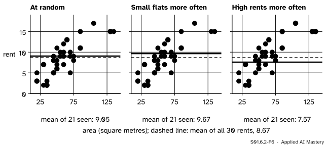
A scraper drops some rents by chance. Whether a rent is lost has nothing to do with the flat. This is missing completely at random, or MCAR.
One agency in Centre leaves rents out of its listings. Whether a rent is lost depends on the district, a column you have for every flat. This is missing at random, or MAR.
Dear flats say “price on request”. Whether a rent is lost depends on the rent itself, the very value you cannot see. This is missing not at random, or MNAR.
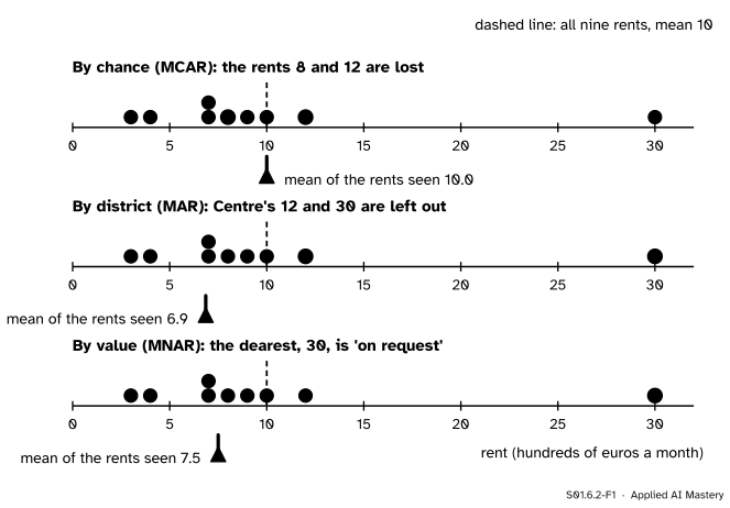
S01.6.2-F1
One column, three reasons for a hole. Lost by chance, the seven rents left still average \(10\). Left out by one district, they average \(6.9\). Hidden because they are dear, they average \(7.5\). The dashed line is the mean of all nine, \(10\).
The names are old and confusing: “missing at random” does not mean random. Remember the stories instead, or better, the question behind them: what decides whether a value goes missing?
Build it up
Step 1. Chance decides (MCAR). If every rent has the same chance of being lost, the seven that survive are a simple random sample of the nine (S01.2.1). One draw can be lucky or unlucky, but there is no lean. Hiding \(8\) and \(12\) leaves \(3, 4, 7, 7, 9, 10, 30\), whose sum is \(70\) and mean \(10\). Hiding \(3\) and \(4\) instead leaves a mean of \({83/7} = 11.86\). Over all \(36\) ways of hiding two of the nine rents, the means of the seven left average exactly \(10\). Holes of this kind add sampling variability and no bias (S01.2.2).
Step 2. The hidden value decides (MNAR). If dear rents are the ones that go missing, the survivors lean cheap every time. Hiding the penthouse’s \(30\) leaves eight rents that sum to \(60\), a mean of \(7.5\). Hide it again tomorrow and you get \(7.5\) again: this is bias, the non-response of S01.2.4 one cell at a time.
Step 3. A known column decides (MAR). Suppose one agency, which handles Centre, leaves rents out. Centre’s rents are \(12\), \(30\) and \(9\). If the agency hides two of them, the seen rents are short of Centre, the dearest district, so their mean leans low. But the district of every flat is still in the table. Inside each district, the chance of a hole is the same for every flat, so the rents seen in a district are a fair sample of that district.
Step 4. Repair MAR with weights. Since the district shares of the table are known, compute a mean for each district from the rents seen there, then weight each district mean by the district’s share of all rows, holes included (the weighted mean of S01.2.3). Each district then counts for what it really is in the table, not for what survived.
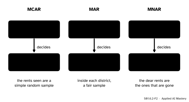
S01.6.2-F2
What decides a hole. Under MCAR it is chance alone. Under MAR it is a column you have. Under MNAR it is the hidden value itself.
The formal statement
NoteDefinition: the three mechanisms
Let \(m_i = 1\) when the value of row \(i\) in a column is missing. The missingness mechanism is the rule that sets the chance that \(m_i = 1\).
MCAR: the chance is the same for every row.
MAR: the chance may differ between rows, but only through columns that are observed: inside any group of rows that agree on those columns, it is the same.
MNAR: neither holds; the chance depends on the missing value itself, or on something that was not recorded.
The reweighted mean. Group the rows by an observed column with groups \(g\). Write \(n_g\) for the number of all rows in group \(g\) and \(w_g = {n_g / n}\) for its share, and \(\bar{x}_{g}\) for the mean of the values seen in group \(g\). The reweighted mean is
\[
\bar{x}_w = \sum_{g} w_g\, \bar{x}_{g}.
\]
Why it aims at the right target. The mean of a complete column is its total over \(n\), and the total is the sum of the group totals. Group \(g\)’s total is \(n_g\) times its complete mean \(\mu_g\), so
The reweighted mean puts \(\bar{x}_g\) where this formula has \(\mu_g\). Under MAR (by groups \(g\)), the values seen in group \(g\) are a simple random sample of that group, so \(\bar{x}_g\) has no lean and averages to \(\mu_g\) over repeated holes; the weights, known exactly, do the rest. Under MCAR the same holds, and the plain mean of the values seen works too.
Go deeper: why no weighting can repair MNAR
Under MNAR the lean is inside the groups. In the city simulation below, Centre’s dear rents are the ones that go missing, so Centre’s mean of the rents seen is too low, and so is every weighted combination that uses it. Weights move whole groups up or down; they cannot fix a group mean that is itself biased. Only information about the hidden values (a follow-up survey, a model of who says “price on request”, or an honest range of possible answers) can, and S08.7 takes this up.
What the table can show, and what it cannot. Compare the other columns between rows with a hole and rows without. If they differ, the holes are not MCAR. But MAR and MNAR can leave the same signal, and nothing in the cells you can see can tell you whether the hidden values themselves decided. If a column has no relation to any other, MNAR leaves no trace at all: the eight rents left after hiding the penthouse, \(3, 4, 7, 7, 8, 9, 10, 12\), look like an ordinary column of rents. Whether data are MAR or MNAR is an assumption, argued from how the data were collected.
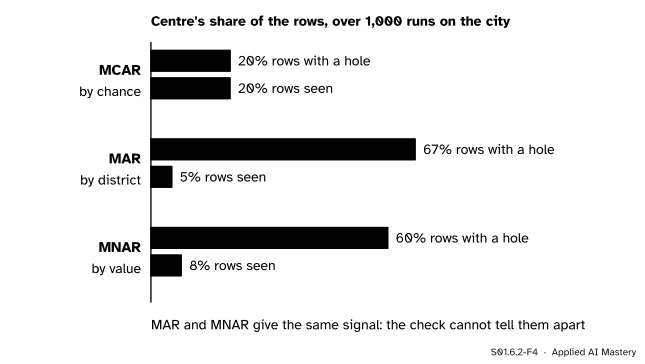
S01.6.2-F4
The check on another column, averaged over \(1{,}000\) runs on the city. Under MCAR, Centre’s share is the same among rows with and without a hole. Under MAR and MNAR it is far higher among the holes, and the two look alike.
Worked example
The agency hides two of Centre’s three rents. Compare the plain mean of the rents seen with the mean reweighted by district. Each district holds three of the nine rows, so each weight is \(w_g = {3/9} = {1/3}\). South’s rents are \(3, 8, 4\) (mean \(5\)) and North’s are \(7, 10, 7\) (mean \(8\)); together they sum to \(39\). Centre keeps one of \(12\), \(30\) and \(9\).
S01.6.2-F3
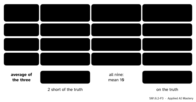
The three ways the agency can hide two of Centre’s rents. The plain means average \(8.00\), short by \(2\). The reweighted means average \(10.00\), the mean of all nine.
Keep Centre’s 12. The seven rents seen sum to \({39 + 12} = 51\), mean \({51/7} = 7.29\). The district means are \(5\), \(8\) and \(12\), and \({\tfrac13(5 + 8 + 12)} = {25/3} = 8.33\).
Average over the three ways. Plain: \({(51 + 69 + 48)/21} = {168/21} = 8.00\). Reweighted: \({(25 + 43 + 22)/9} = {90/9} = 10.00\), exactly the mean of all nine rents. Any single answer can be far off, since one Centre rent stands in for three, but the reweighted mean has no lean, while the plain mean is \(2\) short on average.
Code
The hand-worked cases first, from scratch.
from itertools import combinationsrents = [7, 12, 3, 10, 30, 8, 9, 4, 7] # F1 to F9district = ["North", "Centre", "South", "North", "Centre", "South", "Centre", "South", "North"]mean =lambda values: sum(values) /len(values)# MCAR: every way of hiding two of the nine is equally likelymeans_mcar = [mean([r for k, r inenumerate(rents) if k notin pair]) for pair in combinations(range(9), 2)]print(len(means_mcar), "ways; their means average", round(mean(means_mcar), 6))# MNAR: the dearest rent is on requestprint("penthouse hidden:", mean([r for r in rents if r !=30]))# MAR: the agency hides two of Centre's three rentscentre = [k for k inrange(9) if district[k] =="Centre"]plain, reweighted = [], []for hidden in combinations(centre, 2): seen = [k for k inrange(9) if k notin hidden] plain.append(mean([rents[k] for k in seen])) group_means = [mean([rents[k] for k in seen if district[k] == g]) for g in ("South", "North", "Centre")] reweighted.append(sum(m /3for m in group_means)) # each district is 3 of the 9 rowsprint("plain:", [round(p, 2) for p in plain], "average", round(mean(plain), 2))print("reweighted:", [round(w, 2) for w in reweighted], "average", round(mean(reweighted), 2))
36 ways; their means average 10.0
penthouse hidden: 7.5
plain: [6.86, 9.86, 7.29] average 8.0
reweighted: [7.33, 14.33, 8.33] average 10.0
Now the city of course S01: \(500\) flats, half in South, three tenths in North and a fifth in Centre, with mean rent \(8.3\). Each run hides rents by one of three rules, which all hide about a quarter of the rents: every rent with chance \(0.25\) (MCAR); Centre’s rents with chance \(0.8\) and the others with \(0.1\) (MAR); rents above \(12\) with chance \(0.8\) and the others with \(0.1\) (MNAR). Over \(1{,}000\) runs we average the plain and the reweighted means, as S01.2.2 averaged repeated samples.
import numpy as nprng = np.random.default_rng(0) # the city, built as in every S01 lessonparts, names = [], []for name, size, mu in (("South", 250, 5.0), ("North", 150, 8.0), ("Centre", 100, 17.0)): draws = rng.gamma(9.0, 1.0, size) parts.append(draws * mu / draws.mean()) names += [name] * sizecity, names = np.concatenate(parts), np.array(names)shares = {"South": 0.5, "North": 0.3, "Centre": 0.2}rules = {"MCAR": np.full(500, 0.25),"MAR": np.where(names =="Centre", 0.8, 0.1),"MNAR": np.where(city >12, 0.8, 0.1)}result = {}for rule, chance in rules.items(): rng = np.random.default_rng(1) # the same seed for each rule plain, reweighted, centre_holes, centre_seen = [], [], [], []for _ inrange(1000): seen = rng.random(500) >= chance plain.append(city[seen].mean()) reweighted.append(sum(w * city[seen & (names == g)].mean() for g, w in shares.items())) centre_holes.append(np.mean(names[~seen] =="Centre")) centre_seen.append(np.mean(names[seen] =="Centre")) result[rule] = [np.mean(v) for v in (plain, reweighted, centre_holes, centre_seen)]print(f"{rule:5s} plain {result[rule][0]:.2f} reweighted {result[rule][1]:.2f} "f"Centre among holes {result[rule][2]:.0%}, among rows seen {result[rule][3]:.0%}")print("city mean", round(city.mean(), 2))
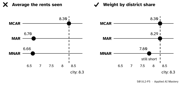
MCAR  plain 8.30  reweighted 8.30  Centre among holes 20%, among rows seen 20%
MAR   plain 6.70  reweighted 8.29  Centre among holes 67%, among rows seen 5%
MNAR  plain 6.66  reweighted 7.80  Centre among holes 60%, among rows seen 8%
city mean 8.3
To two decimals (your last digit may differ with another version of NumPy): under MCAR both means average \(8.30\); under MAR the plain mean averages \(6.70\) and the reweighted one \(8.29\); under MNAR the plain mean averages \(6.66\) and reweighting only lifts it to \(7.80\), still \(0.5\) short. The check on districts flags MAR and MNAR alike: Centre is about two thirds of the rows with a hole in both, against a fifth of all rows.
Explore
S01.6-X1
Missingness machine
Choose how rents go missing and how many, then press New draw a few times. At random, the mean wobbles around the truth; when small flats or high rents lose their rents, it leans the same way on almost every draw. Then switch to Fill with the mean and watch the spread and the correlation.
Pitfalls
S01.6.2-F5
Wrong beside right. The plain mean of the rents seen is right only under MCAR. Reweighting by district repairs MAR, and MNAR stays short.
“Only a few values are missing, so it cannot matter.”
The bias depends on which values are missing, not only on how many. Hiding one rent of nine, the penthouse’s, moves the mean from \(10\) to \(7.5\). A machine-learning model trained on rows where high earners left their income blank learns from a population with the rich left out.
“Missing at random means the holes are random.”
MAR means random inside groups defined by columns you have. Across the whole table, MAR holes can lean as hard as MNAR ones: the plain mean under MAR averaged \(6.70\) against the city’s \(8.3\). The difference is that MAR can be repaired with what the table holds.
“The holes differ by district, so I know the mechanism is MAR.”
A difference between rows with and without holes rules out MCAR, nothing more. MNAR gave the same signal in the city. Deciding between MAR and MNAR takes knowledge of how the data were collected; treat any claim of MAR as an assumption and say so in your report.
Check yourself
Recall
1. In one question, how do you tell MCAR, MAR and MNAR apart?
Show answer
Ask what decides whether a value goes missing: chance alone (MCAR), columns you have (MAR), or the missing value itself or something unrecorded (MNAR).
2. What kind of sample of the column do the values seen form under MCAR?
Show answer
A simple random sample: more variability than the full column, and no bias.
3. Hiding the penthouse’s rent of \(30\) moves the mean of the nine rents from \(10\) to what, and which mechanism is this?
Show answer
To \({60/8} = 7.5\). The rent is hidden because it is high, so it is MNAR.
4. Write the reweighted mean, and say what the weights are.
Show answer
\(\bar{x}_w = {\sum_g w_g \bar{x}_g}\), where \(\bar{x}_g\) is the mean of the values seen in group \(g\) and \(w_g = {n_g/n}\) is group \(g\)’s share of all rows, holes included.
5. Rows with holes contain far more Centre flats than rows without. What can you conclude?
Show answer
That the holes are not MCAR. You cannot tell from the table whether they are MAR or MNAR.
Exercises
1.★ Classify each story. (a) A sensor fails at random moments. (b) Older respondents skip an online question more often, and age is recorded for everyone. (c) People with high debts leave the debt question blank.
Show solution
(a) MCAR: chance alone decides. (b) MAR: the chance depends on age, a column you have. (c) MNAR: the chance depends on the hidden debt itself.
2.★★ A survey has \(60\) students and \(40\) staff. Every staff member answers a question on commuting time; only \(15\) of the students do, at random among students. The students who answer average \(20\) minutes and the staff \(40\). Compute the plain mean of the answers and the mean reweighted by group.
Show solution
Plain: \({(15 \times 20 + 40 \times 40)/(15 + 40)} = {(300 + 1600)/55} = {1900/55} = 34.55\) minutes. Reweighted with the shares of all \(100\) people: \({0.6 \times 20 + 0.4 \times 40} = {12 + 16} = 28\) minutes. The plain mean lets the staff count for \({40/55} = 73\%\) instead of \(40\%\).
3.★★★ Hiding any two of the nine rents at random, show that the mean of the seven left averages exactly \(10\) over all \(36\) ways. Use a counting argument, not a list.
Show solution
Each rent is left in by \(\binom{8}{2} = 28\) of the \(36\) ways (the two hidden rents are chosen from the other eight). So the seven-rent sums, added over all \(36\) ways, give \(28\) times the total of the nine rents, and the means, added over the same ways, give that divided by \(7\):
The average over the \(36\) ways is \({360/36} = 10\), the mean of all nine.
Summary card
What decides a hole decides what the values left can tell you.
S01.6.2-F1
Chance, a known column, or the value itself.
MCAR: same chance for every row; the values seen are a simple random sample.
MAR: chance depends only on observed columns; fair inside groups; repair with \(\bar{x}_w = {\sum_g w_g \bar{x}_g}\).
MNAR: chance depends on the hidden value; no weighting by observed columns repairs it.
Checks on other columns can rule out MCAR, never MNAR.
Sources and next steps
Sources. Each was opened and checked against this lesson on 12 November 2026.
Stef van Buuren, Flexible Imputation of Missing Data, second edition, Section 1.2, Concepts of MCAR, MAR and MNAR. MCAR as the same chance of being missing for all cases, MAR as the same chance only within groups defined by the observed data (illustrated by a weighing scale that fails more often on a soft surface), and MNAR as neither.
Andrew Gelman and Jennifer Hill, Data Analysis Using Regression and Multilevel/Hierarchical Models, Chapter 25, Missing-data imputation, Section 25.1. The four mechanisms from completely at random to missingness that depends on the missing value itself (higher earners less likely to reveal their earnings), and the general impossibility of proving that data are missing at random. Section 25.2 describes the nonresponse weighting that the reweighted mean is a simple case of.
Next.S01.6.3 Dropping rows and columns prices the most common response to holes, deleting them, using what this lesson says about each mechanism.