The mean is the balance point of a dot plot. See why the deviations from it cancel, prove that it is the constant with the smallest squared error, rebuild it from group means with a weighted mean, and watch one penthouse drag it.
Compute the mean of a column by hand and in code, and read it as the balance point of a dot plot.
Prove that the deviations from the mean add up to zero.
Show by algebra that the mean is the constant with the smallest sum of squared deviations, and link this to the baseline prediction of a regression model.
Rebuild an overall mean from group means and group shares as a weighted mean.
Explain why a single extreme value can move the mean as far as it likes.
In review. The maths and code on this page are checked by automated tests on every change, but an independent reader has not signed it off yet. Spot a mistake or a confusing step? Tell us.
The question
Nine flats rent for 3, 4, 7, 7, 8, 9, 10, 12 and 30 hundred euros a month. Asked for one number that stands for “the rent here”, most people add them up and divide by nine: 10. Yet six of the nine flats pay less than 10, and only two pay more. What is the mean really measuring, why does machine learning lean on it so heavily, and what can one expensive flat do to it?
Intuition
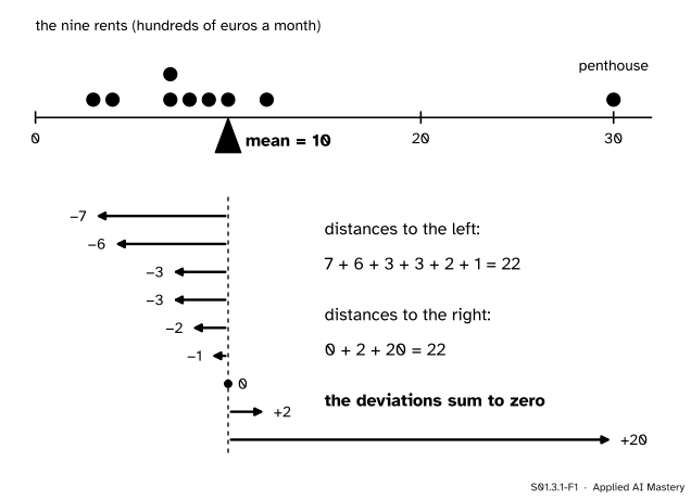
The nine rents come from the flats table of this course, an invented example: nine flats to let, three from each district. Flat F5, the penthouse, pays 30. Put each rent on a number line as a dot of the same weight, and think of the line as a plank. The mean is the point where you could rest the plank on a single support and it would balance.
S01.3.1-F1
The nine rents balance on a support at 10. Each arrow is one flat’s deviation, its distance from the mean with a sign. The six on the left add to 22, and so do the three on the right.
Why 10 and not 8, where the bulk of the dots sit? Because a plank balances when the pulls on each side cancel, and a dot far out pulls hard. The penthouse sits 20 to the right of 10; it alone outweighs the five closest flats on the left put together. Six small distances on one side, one huge one on the other: the support has to sit where they cancel, and that is 10.
So the mean is not “the typical value”. It is the centre of mass of the values, and every value counts in proportion to how far out it is.
Build it up
Step 1. A sum over a count. You have used the mean since S01.2 as “add them up, divide by how many”. For the rents the sum is \(90\) and the count is \(9\), so the mean is \({90/9 = 10}\), in hundreds of euros.
Step 2. Measure every value from the mean. Subtract 10 from each rent. The results −7, −6, −3, −3, −2, −1, 0, 2, 20 are the deviations of the figure above. They are the arrows.
Step 3. The deviations cancel. Add them: \({-22 + 22 = 0}\). That is what balance means, and it is no accident of these numbers: the formal section proves it for any list.
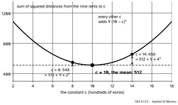
Step 4. Score a guess. Suppose you must predict every rent with one number \(c\), and each miss costs its square. The total cost is the sum of squared distances from the rents to \(c\). Try a few values of \(c\) and plot the cost.
S01.3.1-F2
The cost of predicting every rent with one constant \(c\). It is lowest at the mean, and every other \(c\) pays the same floor of 512 plus an extra \({9\,(10 - c)^2}\).
The curve has its floor at \({c = 10}\). Even the median, 8, the middle of the sorted rents, costs more: \(548\) against \(512\). The formal section shows that the extra is always \(n\) times the squared distance from \(c\) to the mean.
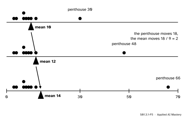
Step 5. Pull on one end. Move the penthouse further out. The other eight dots stay where they are, but the support has to slide right to keep the plank level.
S01.3.1-F5
Moving one value by 18 moves the mean by \({18/9 = 2}\), every time. There is no limit: push the penthouse far enough and the mean goes wherever you like.
The formal statement
NoteDefinition: the mean
For values \({x_1, \dots, x_n}\), the mean is
\[
\bar{x} = \frac{1}{n}\sum_{i=1}^{n} x_i .
\]
The deviation of value \(i\) is \({x_i - \bar{x}}\). When the values are a sample from a population (S01.2.1), \(\bar{x}\) is a statistic; the population mean is written \(\mu\).
Result 1: the deviations add to zero. Split the sum of deviations into two sums, then use the definition, which says that \({\sum x_i = n\bar{x}}\):
The second sum adds the same number \(\bar{x}\) to itself \(n\) times. This is the balance of the anchor figure: the negative deviations exactly cancel the positive ones.
Result 2: the mean is the best constant under squared error. For any number \(c\),
Why. Write each distance to \(c\) as a distance to the mean plus a fixed step: \({x_i - c} = {(x_i - \bar{x})} + {(\bar{x} - c)}\). Square it, using \({(a + b)^2} = {a^2 + 2ab + b^2}\):
Now add over \(i\). The first terms give \({\sum (x_i - \bar{x})^2}\). In the middle terms the factor \({2(\bar{x} - c)}\) is the same for every \(i\), so it comes out of the sum, leaving \({2(\bar{x} - c)\sum (x_i - \bar{x})}\), which is zero by Result 1. The last term is the same for every \(i\), so it adds up to \({n(\bar{x} - c)^2}\). That proves the identity.
The first part on the right does not depend on \(c\). The second part is a square times \(n\), so it is never negative, and it is zero only when \({c = \bar{x}}\). So no constant has a smaller sum of squared deviations than the mean. For the rents, \({\sum (x_i - 10)^2 = 512}\), and any other \(c\) adds \({9\,(10 - c)^2}\): the curve of Step 4. No calculus was needed.
This is why the mean is the baseline of regression. A model that ignores its inputs and predicts one number, scored by mean squared error, does best by predicting the mean of its training targets; lesson ML01.7.4 uses that constant as the yardstick every model must beat.
Result 3: the overall mean from group means. Split the \(n\) values into groups \(g\), of sizes \(n_g\) and means \(\bar{x}_g\). The total of group \(g\) is \(n_g \bar{x}_g\), and the overall total is the sum of the group totals. Divide by \(n\):
The overall mean is the weighted mean of the group means, each weighted by its group’s share \(\cparam{w_g}\) of the rows. The shares add to 1. This is the formula S01.2.3 used for strata, \({\mu = \sum_g W_g \mu_g}\), now read the other way: from the parts back to the whole.
Result 4: one value moves the mean by its change over \(n\). Replace \(x_k\) by \({x_k + \Delta}\). The sum grows by \(\Delta\), so the mean grows by \({\Delta / n}\). Since \(\Delta\) can be as large as you like, so can the change in the mean. A summary that one bad value can carry anywhere is called not resistant; the median of the next lesson is the resistant one.
Go deeper: why the balance picture is exact, not a metaphor
A plank with equal weights at \({x_1, \dots, x_n}\) balances on a support at \(c\) when the turning effects on the two sides cancel. The turning effect of a weight is its weight times its signed distance from the support, so the plank balances exactly when \({\sum (x_i - c) = 0}\). Solve for \(c\): \({\sum x_i - nc = 0}\), so \({c = \bar{x}}\). Result 1 is the same statement read backwards. With unequal weights \(w_i\), the balance point is \({\sum w_i x_i / \sum w_i}\), the weighted mean of Result 3.
Worked example
The overall mean rebuilt from the three districts. The nine flats are three from each district. Their district means, from the flats table, are:
South: F3, F6, F8 pay 3, 8 and 4, so the mean is \({15 / 3 = 5}\).
North: F1, F4, F9 pay 7, 10 and 7, so the mean is \({24 / 3 = 8}\).
Centre: F2, F5, F7 pay 12, 30 and 9, so the mean is \({51 / 3 = 17}\).
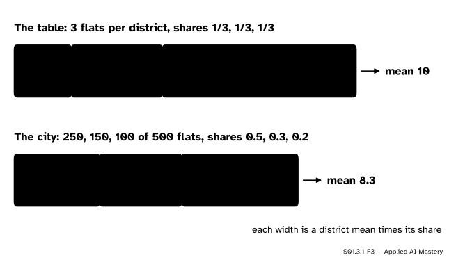
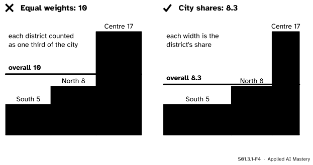
In the table each district holds one third of the rows, so by Result 3 the overall mean is \({\tfrac13 \cdot 5} + {\tfrac13 \cdot 8} + {\tfrac13 \cdot 17} = 10\), as before.
The city those flats came from (S01.2.3) has 500 flats to let: 250 in South, 150 in North and 100 in Centre. Its shares are 0.5, 0.3 and 0.2, and with the same district means:
The same three district means, weighted two ways. Each box’s width is one district’s contribution. The table gives Centre a third of the weight; the city gives it a fifth.
The two answers differ only in the weights. The table over-represents Centre, the dearest district, so its mean of 10 overstates the city’s 8.3. Same means, different shares, different answer.
Code
First from scratch, with a loop, so that nothing is hidden.
rents = [7, 12, 3, 10, 30, 8, 9, 4, 7] # F1 to F9, hundreds of euros a monthtotal =0for x in rents: total += xx_bar = total /len(rents)deviations = [x - x_bar for x in rents]def squared_cost(c, values):"""The sum of squared distances from the values to the constant c."""returnsum((x - c) **2for x in values)print("mean:", x_bar, " sum of deviations:", sum(deviations))for c in (7, 8, 10, 14):print(f"c = {c:>2}: cost {squared_cost(c, rents):.0f}")
mean: 10.0   sum of deviations: 0.0
c =  7: cost 593
c =  8: cost 548
c = 10: cost 512
c = 14: cost 656
Every cost matches \({512 + 9\,(10 - c)^2}\). Now the group means, the weighted means and the penthouse, with NumPy.
import numpy as npdistricts = ["North", "Centre", "South", "North", "Centre", "South", "Centre", "South", "North"]x = np.array(rents, dtype=float)group_means = {g: x[[d == g for d in districts]].mean() for g in ("South", "North", "Centre")}means = np.array(list(group_means.values()))table_mean = np.average(means, weights=[3, 3, 3]) # counts work as weights toocity_mean = np.average(means, weights=[250, 150, 100])print(group_means, " table:", table_mean, " city:", round(city_mean, 2))for penthouse in (30, 48, 66): moved = x.copy() moved[4] = penthouse # F5 is the fifth flatprint(f"penthouse {penthouse}: mean {np.mean(moved):.2f}")print("without the penthouse:", np.mean(np.delete(x, 4)))
{'South': np.float64(5.0), 'North': np.float64(8.0), 'Centre': np.float64(17.0)}  table: 10.0  city: 8.3
penthouse 30: mean 10.00
penthouse 48: mean 12.00
penthouse 66: mean 14.00
without the penthouse: 7.5
numpy.average divides by the sum of the weights, so counts and shares give the same answer. Without the penthouse the mean falls from 10 to 7.5: one flat out of nine moved it by 2.5.
Explore
This module’s interactive, Balance and middle, lives in lesson S01.3.3. There you can drag any rent and watch the balance point slide by one ninth of every move.
Pitfalls
S01.3.1-F4
Wrong beside right. Averaging the three district means treats the districts as equal in size. Weighting each by its share of the city gives the city’s mean. The overall mean is the height of a flat bar with the same total area.
“The overall mean is the mean of the group means.”
Only when the groups are the same size. In the city, South has two and a half times as many flats as Centre, so the plain average of 5, 8 and 17 (which is 10) overstates the city mean of 8.3. Weight each group mean by its share. S01.7 shows that getting the weights wrong can even reverse a comparison.
“The mean is the typical value.”
It is the balance point, and a long tail drags it. Six of the nine flats pay less than the mean of 10, and only two pay more. When a column has a long tail (incomes, house prices, waiting times), quote the median of the next lesson beside the mean, or instead of it.
“The mean is the best single guess, whatever the scoring.”
It is the best guess when misses are scored by their squares. Score them by their size instead (mean absolute error) and the mean loses: the total distance from the rents to 10 is 44, but to the median, 8, it is only 40. The next lesson shows why the median wins that contest. Pick the summary that matches the loss.
“Ratings are coded 1 to 4, so their mean is the average rating.”
A mean adds distances, and an ordinal column such as the energy rating has an order but no distances (S01.1.2). The mean of the codes depends on which codes you chose. Use the median or the mode for such a column.
Check yourself
Recall
1. What is the mean of the nine rents, and how many flats pay less than it?
Show answer
\({90 / 9 = 10}\) hundred euros. Six flats pay less (3, 4, 7, 7, 8 and 9), one pays exactly 10 and two pay more.
2. What do the deviations from the mean always add up to, and why?
Show answer
Zero. Their sum is \({\sum x_i - n\bar{x}}\), and \({\sum x_i = n\bar{x}}\) by the definition of the mean.
3. Which constant \(c\) makes \({\sum (x_i - c)^2}\) as small as possible, and by how much does any other \(c\) exceed that minimum?
Show answer
The mean, \(\bar{x}\). Any other \(c\) adds \({n(\bar{x} - c)^2}\).
4. Three groups have means 5, 8 and 17 and shares 0.5, 0.3 and 0.2. What is the overall mean?
5. One of nine values rises by 18. How far does the mean move?
Show answer
By \({18 / 9 = 2}\), in the same direction.
Exercises
1.★ Find the mean of the eight rents left when the penthouse is removed, list their deviations, and check that the deviations add to zero.
Show solution
The eight rents 3, 4, 7, 7, 8, 9, 10, 12 add to 60, so the mean is \({60 / 8 = 7.5}\). The deviations are −4.5, −3.5, −0.5, −0.5, 0.5, 1.5, 2.5, 4.5. The negative ones add to \({-9}\) and the positive ones to \({+9}\), so the total is 0.
2.★★ (a) A tenth flat joins the nine. What rent must it have for the mean of all ten to be 11? (b) Without adding up nine squares, find \({\sum (x_i - 7)^2}\) for the nine rents, then check it directly.
Show solution
(a) Ten flats with mean 11 have a total of 110. The nine pay 90, so the tenth must pay \({110 - 90 = 20}\).
(b) By Result 2 with \({c = 7}\): \({512 + 9\,(10 - 7)^2} = {512 + 81} = 593\). Directly, the distances from 7 are −4, −3, 0, 0, 1, 2, 3, 5, 23, whose squares are 16, 9, 0, 0, 1, 4, 9, 25 and 529, and these add to 593.
3.★★★ Prove that if every value is changed to \({y_i = a x_i + b}\), then \({\bar{y} = a\bar{x} + b}\). Use it to give the mean rent in euros, and the mean after a service charge of 50 euros is added to every rent.
Show solution
Split the sum and take the constants out:
\[
\begin{aligned}
\bar{y} &= \frac{1}{n}\sum_{i=1}^{n} (a x_i + b) \\
&= \frac{a}{n}\sum_{i=1}^{n} x_i + \frac{1}{n}\cdot nb \\
&= a\bar{x} + b .
\end{aligned}
\]
Rents are in hundreds of euros, so in euros \({a = 100}\), \({b = 0}\) and the mean is 1,000 euros. A service charge of 50 euros is \({b = 0.5}\) hundred euros, so the mean becomes 10.5 hundred euros, or 1,050 euros. The mean follows every change of unit and every shift exactly.
Summary card
The mean is the balance point: the deviations from it cancel.
From groups.\({\bar{x} = \sum_g \cparam{w_g}\,\bar{x}_g}\) with \({\cparam{w_g} = n_g / n}\).
Not resistant. Changing one value by \(\Delta\) moves the mean by \({\Delta / n}\).
Sources and next steps
Sources. Each was opened and checked against this lesson on 12 November 2026.
David Diez, Mine Cetinkaya-Rundel and Christopher Barr, OpenIntro Statistics, 4th edition (free PDF). Section 2.1.2, Dot plots and the mean, defines the sample mean \(\bar{x}\) as the sum of the observations over their number and describes it as the balancing point of the distribution, drawn as a triangle under a dot plot.
NIST/SEMATECH, e-Handbook of Statistical Methods, Section 1.3.5.1, Measures of location: the mean as the sum of the data points over their number, and the warning that extreme values in the tails distort the mean, for which the median is the better estimate of location.
NumPy documentation, numpy.average: the weighted average is the sum of the values times the weights over the sum of the weights, so the weights need not add to 1.