Two ways to be wrong: sampling variability and bias
Repeated samples scatter around their own centre, and a biased method puts that centre off the truth. Measure both with means alone, watch the scatter shrink as samples grow, and see why no sample size repairs a sample drawn from the wrong place.
Tell sampling variability from bias, in the target picture and on a number line of sample means.
Compute the centre, the bias and the scatter of a sampling method from its sample means.
Show that a simple random sample from a frame centres on the frame’s mean, so its bias is the same at every sample size.
Simulate repeated samples from the city and read off how the scatter and the bias change as n grows.
Explain why more rows do not repair rows drawn from the wrong population, in polls and in machine learning.
In review. The maths and code on this page are checked by automated tests on every change, but an independent reader has not signed it off yet. Spot a mistake or a confusing step? Tell us.
The question
In 1936 the Literary Digest collected nearly 2.4 million straw ballots and predicted that Alf Landon would beat Franklin Roosevelt for the American presidency. Roosevelt won with 61 percent of the vote. How can 2.4 million answers be so wrong, and would 24 million have done better?
From the last lesson
1. What makes a sample of size \(n\) a simple random sample?
Show answer
Every set of \(n\) units of the population has the same chance of being the sample.
2. The ten samples of two from the rents 4, 7, 8, 9, 12 have means from 5.5 to 10.5. What do they average?
Show answer
Exactly 8, the population mean \(\mu\), because each flat is in four of the ten samples.
Intuition
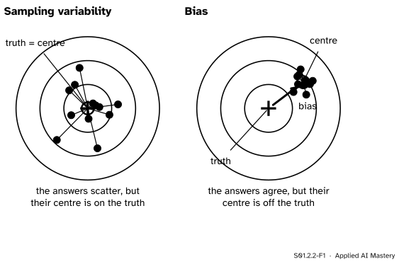
Think of a sampling method as a marksman, and of each sample mean as one shot at the true value \(\ctruth{\mu}\). Fire many shots and two things can go wrong.
S01.2.2-F1
Two ways to be wrong. Left: the sample means scatter, but they are centred on the truth. Right: they agree with each other, but their centre is off the truth. The arrow from the truth to the centre is the bias.
On the left the shots spread out, but their centre sits on the bull’s eye. Any one shot misses, yet the misses lean no particular way. That spread is sampling variability: different samples give different answers just because they hold different units.
On the right the shots cluster tightly, but round the wrong point. Firing more of them only makes the cluster look more convincing. That offset is bias: the method itself leans one way.
You met the same pair in lesson S01.1.4 as the random error and the systematic error of repeated readings. Averaging more readings shrank the random scatter and left the systematic offset alone. Samples behave the same way, and the Literary Digest is the right-hand target.
Build it up
We measure both errors with nothing more than means and distances.
Step 1. A method, repeated. A sampling method is a rule for choosing the sample: “five flats by lot from the whole city”, or “two flats by lot from one website”. Imagine using the rule again and again. Each use gives one sample mean.
Step 2. The centre. The centre of the method is the mean of all those sample means.
Step 3. The bias. The bias is the centre minus the truth. Zero means the method leans neither way.
Step 4. The scatter. The scatter is the average distance of the sample means from their own centre: how far a typical sample mean lands from where the method is aiming.
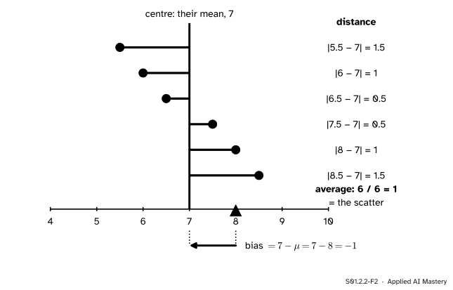
S01.2.2-F2
The two errors measured on six sample means. Their mean, 7, is the centre. The bars are the distances from the centre, which average 1: the scatter. The arrow from the truth, 8, to the centre is the bias, \(-1\).
The six dots in the picture come from a method we work through below. Its centre is 7 and the truth is 8, so its bias is \(-1\). Its distances from the centre average 1, so its scatter is 1.
The formal statement
NoteDefinitions
A sampling method can produce samples whose means are \(\cmodel{\bar{x}}_1, \dots, \cmodel{\bar{x}}_K\): either all its possible samples, each listed as often as it is likely, or many repeats of it. The centre of the method is their mean,
\[
m = \frac{1}{K} \sum_{k=1}^{K} \cmodel{\bar{x}}_k .
\]
The bias of the method is \(\closs{m - \ctruth{\mu}}\), and the method is unbiased when the bias is zero. The scatter is the average distance of the sample means from their centre,
In this course “scatter” is this average distance. Lesson S01.3.3 introduces the standard deviation, the measure that later courses use for the same job.
Result 1: a simple random sample is unbiased. Over all its possible samples the sample mean averages exactly \(\ctruth{\mu}\) (lesson S01.2.1, Consequence 2), so \(m = \mu\) and the bias is zero.
Result 2: a frame has the bias of its own mean, at every sample size. Suppose the sample is drawn by lot, but only from a frame that leaves some units out. Inside the frame this is an ordinary simple random sample, with the frame as its population. So by Result 1, applied to the frame, the centre is the frame’s mean \(\mu_F\), and
\[
\text{bias} = \mu_F - \ctruth{\mu} .
\]
Nothing in that formula depends on \(n\). For the city, a website that lists no flats in Centre has a frame of 250 flats in South with mean 5 and 150 in North with mean 8:
The whole city adds Centre’s 100 flats with mean 17, so \(\mu = {(1250 + 1200 + 1700) / 500} = 8.3\). The bias is \(6.125 - 8.3 = -2.175\), for samples of 4, of 64 or of 400.
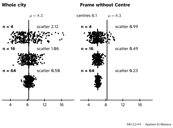
Result 3 (observed): quadruple the sample, halve the scatter. The simulation in the code below draws 1,000 samples at each size. For simple random samples from the whole city the scatter is 2.12 at \(n = 4\), 1.06 at \(n = 16\) and 0.50 at \(n = 64\): it about halves each time \(n\) is multiplied by four. We only observe this here. Lessons M06.11.1 and S02.1 derive the law, for the standard deviation, from probability.
S01.2.2-F4
One thousand sample means at each size; 250 of them are drawn as dots. Left: from the whole city the strips narrow and stay centred on \(\ctruth{\mu} = 8.3\). Right: from a frame without Centre they narrow just as fast, round 6.1.
Go deeper: the average miss is never smaller than the bias
What a user of one sample cares about is the miss \(\abs{\bar{x}_k - \mu}\). Its average over the method combines both errors, and it can never be less than the size of the bias. The size of an average is at most the average of the sizes, because positive and negative terms can cancel inside the sum but not outside it:
The first line uses \(m - \mu = \frac{1}{K}\sum_k \bar{x}_k - \mu\), with the \(\mu\) taken inside the sum \(K\) times and divided by \(K\). So a large sample from the wrong frame, whose scatter is nearly zero, still misses by about 2.175 on average.
Worked example
Two ways to sample two flats from the five. Method A is a simple random sample from all five (rents 4, 7, 8, 9, 12, \(\mu = 8\)). Method B also draws two by lot, but from a website that does not list F2, the dearest flat, so its frame is 4, 7, 8, 9.
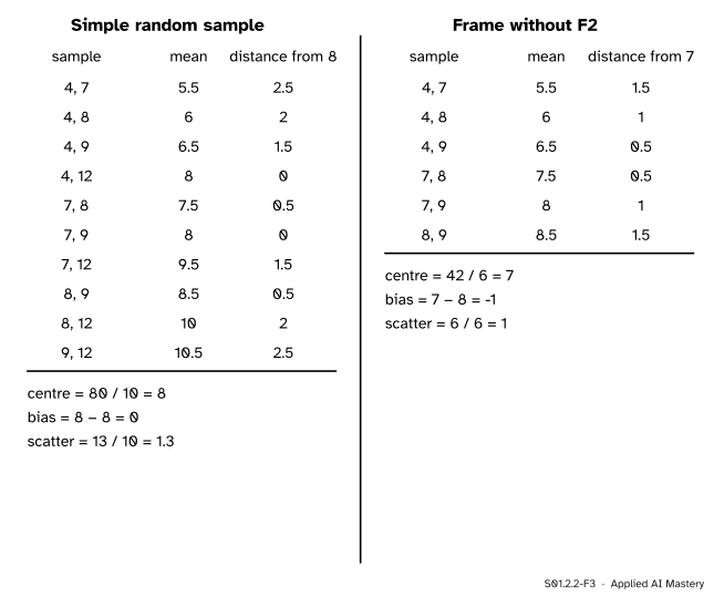
S01.2.2-F3
Both methods worked by hand. A is centred on the truth and scatters by 1.3. B scatters less, by 1, but is centred 1 below the truth.
Method A. Its ten equally likely samples are those of lesson S01.2.1. Their means add to 80, so the centre is \(80 / 10 = 8\) and the bias is \(8 - 8 = 0\). The distances from 8 are 2.5, 2, 1.5, 0, 0.5, 0, 1.5, 0.5, 2 and 2.5, which add to 13, so the scatter is \(13 / 10 = 1.3\).
Method B. There are \(\binom{4}{2} = 6\) samples, with means 5.5, 6, 6.5, 7.5, 8 and 8.5. They add to 42, so the centre is \(42 / 6 = 7\), which is the mean of the frame, \(28 / 4\), as Result 2 says. The bias is \(7 - 8 = -1\). The distances from 7 are 1.5, 1, 0.5, 0.5, 1 and 1.5, which add to 6, so the scatter is \(6 / 6 = 1\).
Look at what the numbers say. The biased method has the smaller scatter, because leaving out the extreme rent of 12 makes the samples more alike. Judged by how well its answers agree, Method B looks better. Even its average miss from the truth, \(7/6 \approx 1.17\), is a little below A’s 1.3, but only because samples of two are tiny. Make the samples larger and A’s misses shrink towards 0, while B’s can never fall below 1, the size of its bias. Scatter shrinks as \(n\) grows; bias does not.
Code
First the hand calculation, from scratch, so that the three definitions are code.
import itertoolsimport numpy as npdef centre_bias_scatter(means, mu): m =sum(means) /len(means) scatter =sum(abs(x - m) for x in means) /len(means)return m, m - mu, scatterfive = [4, 7, 8, 9, 12]A = [(a + b) /2for a, b in itertools.combinations(five, 2)]B = [(a + b) /2for a, b in itertools.combinations(five[:4], 2)]print("A: centre, bias, scatter =", centre_bias_scatter(A, 8))print("B: centre, bias, scatter =", centre_bias_scatter(B, 8))
A: centre, bias, scatter = (8.0, 0.0, 1.3)
B: centre, bias, scatter = (7.0, -1.0, 1.0)
Now the city. Every lesson of the course builds its 500 rents the same way, from seed 0, so that the three district means are exactly 5, 8 and 17.
rng = np.random.default_rng(0)sizes = {"South": 250, "North": 150, "Centre": 100}district_mean = {"South": 5, "North": 8, "Centre": 17}rents, district = [], []for name in ("South", "North", "Centre"): draws = rng.gamma(9.0, 1.0, sizes[name]) rents.append(draws * district_mean[name] / draws.mean()) district += [name] * sizes[name]rents, district = np.concatenate(rents), np.array(district)frame = rents[district !="Centre"]mu, mu_frame = rents.mean(), frame.mean()print(f"mu = {mu:.3f}, frame mean = {mu_frame:.3f}, bias of the frame = {mu_frame - mu:.3f}")
mu = 8.300, frame mean = 6.125, bias of the frame = -2.175
Draw 1,000 simple random samples at each size, from the whole city and from the frame, and measure each method.
rng = np.random.default_rng(3)results = {}for n in (4, 16, 64): whole = np.array([rng.choice(rents, n, replace=False).mean() for _ inrange(1000)]) part = np.array([rng.choice(frame, n, replace=False).mean() for _ inrange(1000)]) results[n] = (centre_bias_scatter(whole, mu), centre_bias_scatter(part, mu)) (cw, bw, sw), (cp, bp, sp) = results[n]print(f"n = {n:2d} whole city: centre {cw:.2f}, bias {bw:+.2f}, scatter {sw:.2f}"f" frame: centre {cp:.2f}, bias {bp:+.2f}, scatter {sp:.2f}")
n =  4  whole city: centre 8.30, bias +0.00, scatter 2.12   frame: centre 6.07, bias -2.23, scatter 0.99
n = 16  whole city: centre 8.33, bias +0.03, scatter 1.06   frame: centre 6.14, bias -2.16, scatter 0.49
n = 64  whole city: centre 8.33, bias +0.03, scatter 0.50   frame: centre 6.13, bias -2.17, scatter 0.23
The centres from the whole city sit within a few hundredths of 8.3, which is simulation noise. The frame’s centres sit near 6.1 at every \(n\), its bias about \(-2.2\), while its scatter halves just as the whole city’s does. The numbers are rounded; another random generator would move their last digits but not the pattern. The library has no special call for this: rng.choice with replace=False (lesson S01.2.1) and numpy.mean are all a simulation needs.
Explore
S01.2-X1
Sampling bench
Choose how the flats are chosen and a sample size, then draw sample after sample. Compare the centre and the scatter of each method at sizes 2, 4, 8 and 16: which number shrinks, and which stays put?
The 48 flats of the bench are invented, with rents that average exactly 8 and rise towards the top right. By lot is a simple random sample. Near the corner draws by lot from the 24 flats nearest the bottom-left corner only, a frame like the website without Centre. Dear flats answer more asks flats by lot, but a flat answers with a chance that grows with its rent, which lesson S01.2.4 calls non-response.
Pitfalls
S01.2.2-F5
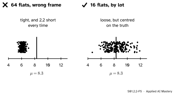
Wrong beside right. Sixty-four flats from a frame without Centre give tight answers that are all too low. Sixteen flats drawn by lot from the whole city scatter more, but around the truth.
“A big enough sample cannot be biased.”
Size shrinks the scatter only. The Literary Digest mailed about 10 million ballots and got nearly 2.4 million back, and it predicted that Roosevelt would get 41 percent of the vote. George Gallup asked far fewer people (one contemporary account puts it at 125,000, about a twentieth of the Digest’s returns), chosen to match the make-up of the voters, and named the right winner. In machine learning the same holds: a model trained on a million rows drawn from the wrong population learns that population well and the right one badly. More rows do not fix where the rows came from (dataset shift, E05.4).
“The answers agree with each other, so they must be right.”
Agreement measures scatter, not bias. In the worked example the biased Method B had the smaller scatter. A tight cluster of polls, or of validation scores from one source, can be tightly wrong.
“An unbiased method gives the right answer.”
It gives the right answer on average over samples. You hold one sample. With four flats drawn by lot from the city, a sample mean misses its centre by 2.12 on average. Unbiased means the misses do not lean one way; it does not mean they are small.
Check yourself
Recall
1. In the target picture, which error is the spread of the shots and which is the offset of their centre?
Show answer
The spread is sampling variability; the offset of the centre from the truth is bias.
2. How are the centre, the bias and the scatter of a sampling method computed?
Show answer
The centre is the mean of the sample means. The bias is the centre minus \(\mu\). The scatter is the average distance of the sample means from their centre.
3. What is the bias of a simple random sample drawn from a frame with mean \(\mu_F\), and how does it depend on \(n\)?
Show answer
\(\mu_F - \mu\), the same at every sample size.
4. In the city simulation, roughly what happens to the scatter of simple random samples when \(n\) is multiplied by four?
Show answer
It about halves: 2.12 at \(n = 4\), 1.06 at \(n = 16\), 0.50 at \(n = 64\).
5. Why did 2.4 million ballots not save the Literary Digest?
Show answer
Because its error was bias, not scatter. A larger sample from the same method lands ever more tightly round the same wrong centre.
Exercises
1.★ A population of four flats has rents 3, 7, 9 and 13. Simple random samples of two have means 5, 6, 8, 8, 10 and 11. Find the centre, the bias and the scatter.
Show solution
\(\mu = 32 / 4 = 8\). The means add to 48, so the centre is \(48 / 6 = 8\) and the bias is 0. The distances from 8 are 3, 2, 0, 0, 2 and 3, which add to 10, so the scatter is \(10 / 6 \approx 1.67\).
2.★★ A website lists four of the five flats but not F8, the cheapest (rent 4). Two flats are drawn by lot from the website. Find the centre, the bias and the scatter, and check the centre against Result 2.
Show solution
The frame is 7, 8, 9, 12. The six samples have means 7.5, 8, 9.5, 8.5, 10 and 10.5, which add to 54, so the centre is \(54 / 6 = 9\). Result 2 predicts the frame’s mean, \(36 / 4 = 9\). The bias is \(9 - 8 = +1\). The distances from 9 are 1.5, 1, 0.5, 0.5, 1 and 1.5, which add to 6, so the scatter is 1.
3.★★★ A website lists every flat of the city except those in North. (a) Find the mean of its frame and the bias of samples drawn by lot from it. (b) For Method B of the worked example, compute the average miss \(\abs{\bar{x} - \mu}\) and check that it is at least the size of the bias.
Show solution
(a) The frame holds 250 flats in South with mean 5 and 100 in Centre with mean 17:
The bias is \(8.43 - 8.3 \approx +0.13\) at every \(n\). Leaving out North, whose mean of 8 is close to \(\mu\), does little harm here; leaving out Centre did a great deal.
(b) The six means 5.5, 6, 6.5, 7.5, 8 and 8.5 miss \(\mu = 8\) by 2.5, 2, 1.5, 0.5, 0 and 0.5, which add to 7. The average miss is \(7 / 6 \approx 1.17\), which is at least \(\abs{-1} = 1\).
Summary card
Scatter shrinks with more data; bias does not.
S01.2.2-F1
Spread round the truth; tight but off it.
Centre\(m\): the mean of the sample means. Bias:\(m - \mu\).
Scatter: the average of \(\abs{\bar{x}_k - m}\).
Simple random sample: bias 0. From a frame: bias \(\mu_F - \mu\) at every \(n\).
Observed: multiply \(n\) by four and the scatter about halves.
Sources and next steps
Sources. Each was opened and checked against this lesson on 12 November 2026.
Dominic Lusinchi, “President” Landon and the 1936 Literary Digest poll: were automobile and telephone owners to blame?, Social Science History 36(1), 2012. About 10 million ballots mailed and nearly 2.4 million returned (24 percent); the forecast of 54 percent for Landon and 41 for Roosevelt against Roosevelt’s 61 percent; the reanalysis showing that non-response was the main culprit; Gallup’s forecast of 55.7 percent of the two-party vote; and the figure of 125,000 for Gallup’s sample, which the article attributes to one source (Robinson 1937).
David Diez, Mine Cetinkaya-Rundel and Christopher Barr, OpenIntro Statistics, 4th edition, Section 1.3.3: random sampling reduces bias, and non-response and convenience samples bring it back.
Barbara Illowsky and Susan Dean, Introductory Statistics 2e, OpenStax, Section 1.2: sampling bias, sampling error, and the rule that larger samples have smaller sampling error.