When one column is a category, compare the groups side by side: their sizes, means, medians and boxplots. When both are categories, tally a two-way table and read its joint, marginal and conditional proportions, comparing rows to see whether the columns go together.
Compare a numerical column across groups by their sizes, means, medians and side-by-side boxplots.
Tally a two-way table of counts by hand, with its row and column totals.
Compute joint, marginal and conditional proportions from a two-way table, and tell a row proportion from a column proportion.
Decide whether two categorical columns are associated by comparing the rows’ conditional proportions.
In review. The maths and code on this page are checked by automated tests on every change, but an independent reader has not signed it off yet. Spot a mistake or a confusing step? Tell us.
The question
Do flats in the Centre cost more than flats in the South? Is a balcony more common in one district than another? Neither question fits the last three lessons, because a district is a label, not a number: there is nothing to put on an axis and no \(r\) to compute. Yet these are the most common questions asked of a table, and in machine learning every classification problem asks one: does this feature look different in one class than in another?
From the last lesson
1. What is \(r\) for \(y = x^2\) on \(x = -2, \dots, 2\), and why?
Show answer
Exactly \(0\): the products of deviations cancel in pairs, because \(r\) measures only straight-line association.
2. How is Spearman’s rank correlation computed, and how are ties handled?
Show answer
Rank each column and compute Pearson’s \(r\) on the ranks; tied values share the average of their ranks.
Intuition
When one column is a number and the other a category, give each category its own strip and lay the strips side by side. Then compare them the way S01.3 and S01.4 taught you to describe one column: how many values, where the centre is, how wide the spread.
S01.5.4-F1
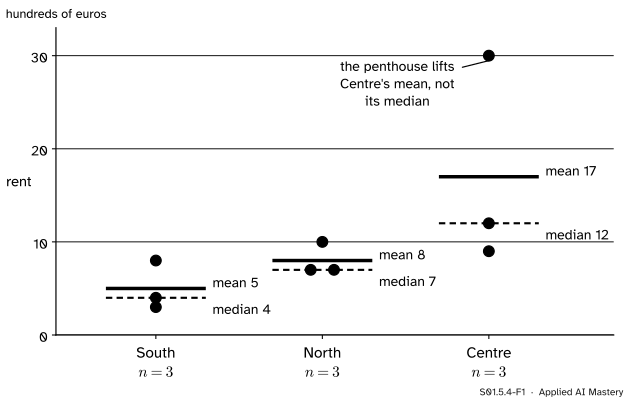
Rent by district for the nine flats of the course’s invented table. Each group’s mean (solid) and median (dashed) sit on its strip.
The strips tell a clear story with a caveat. Rent rises from South to North to Centre: medians 4, 7 and 12. The Centre’s mean of 17 overstates its typical flat, because one of its three flats is the penthouse. And every group holds only three flats, so the picture would shift with any one of them. Always state the group sizes beside the group summaries.
Build it up
Step 1. A number against a category: one summary per group. Split the rows by group and summarise each part. For the flats, the group means are 5, 8 and 17. Because the three groups have three flats each, the overall mean 10 is the plain average of the three group means; with unequal groups it would be the weighted mean of S01.2.3, each group mean weighted by its share of the rows.
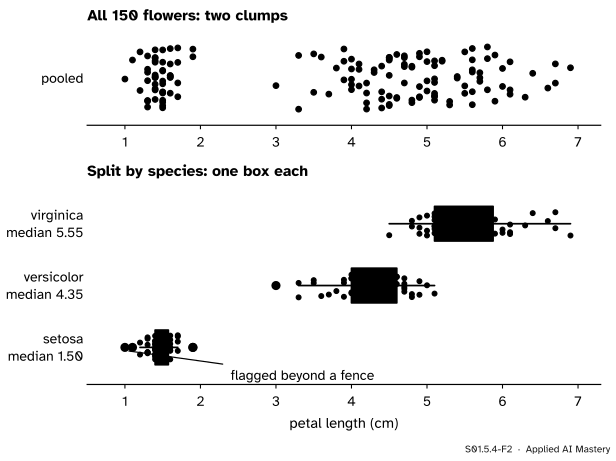
Step 2. Side-by-side boxplots for larger groups. Three values make a poor box. With more, draw one boxplot per group (S01.4.3) on a shared axis. The S01.4 explorer found two clumps in the iris petal lengths. Split them by species and the clumps are explained.
S01.5.4-F2
Petal lengths of the 150 iris flowers in scikit-learn’s copy of the data. Pooled, two clumps; split by species, the small clump is setosa and the large one is versicolor and virginica, overlapping.
The small clump is all setosa, 1.0 to 1.9 cm. The large one is two species, versicolor (3.0 to 5.1) and virginica (4.5 to 6.9), which overlap between 4.5 and 5.1. A clump in one column is often a group hiding in another column.
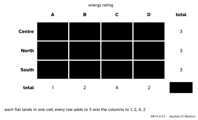
Step 3. A category against a category: count the pairs. For district and energy rating, make a grid with one row per district and one column per rating, and drop each flat into its cell. The result is a two-way table of counts.
Step 4. Turn counts into proportions three ways. A count divided by the grand total, by its row’s total, or by its column’s total answers three different questions. The next section names them.
The formal statement
Write \(n_{gk}\) for the count in row \(g\) and column \(k\) of a two-way table, \({n_{g\cdot}}\) for the total of row \(g\), \({n_{\cdot k}}\) for the total of column \(k\), and \(n\) for the grand total.
NoteDefinition: three proportions in a two-way table
The joint proportion of a cell is \({n_{gk} / n}\): its share of all rows.
The marginal proportion of a row is \({n_{g\cdot} / n}\), and of a column \({n_{\cdot k} / n}\): the totals in the margins, as shares.
The conditional proportion of column \(k\) within row \(g\) is \({n_{gk} / n_{g\cdot}}\): the share inside one row. Dividing by a column total instead gives the share within a column.
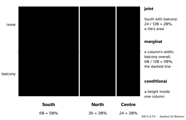
The course’s second table is invented: 120 flats listed for rent, by district and by whether they have a balcony. Its district mix, 60 in South, 36 in North and 24 in Centre, is the city’s 50, 30 and 20 percent.
S01.5.4-F4
120 invented listings as a mosaic. Column widths are the marginal shares of the districts, tile heights the conditional shares of a balcony within each district, and tile areas the joint shares.
The margin is a weighted mean of the rows. Every listing with a balcony sits in exactly one row, so the column total is the sum of its cells. Divide by \(n\) and write each cell as its row total times its conditional proportion:
Association. Two categorical columns are not associated in a table when every row has the same conditional proportions. Then, by the identity, each row’s share equals the margin’s: a weighted mean of equal numbers is that number. When the rows differ, the columns are associated: knowing the district changes what you expect about the balcony. Here the rows read 40, 50 and 75 percent against 50 overall, so district and balcony are associated in these listings. (Whether such a gap could arise by chance is a question for S02; M06.3.1 reads the same table as probabilities.)
Worked example
Tally the flats by district and rating. Read the table row by row and drop each flat into its cell: F1 is North and C, F2 Centre and B, F3 South and D, F4 North and B, F5 Centre and A, F6 South and C, F7 Centre and D, F8 South and C, F9 North and C.
S01.5.4-F3
The two-way table of district by rating, tallied flat by flat, with its margins.
The row totals are 3 each, by the design of the table, and the column totals 1, 2, 4 and 2 are the counts of S01.1.2. Three proportions from it:
Joint. North and C: \({2 / 9} = 22.2\) percent of all flats.
Conditional within a row. Of North’s flats, \({2 / 3} = 66.7\) percent are rated C.
Conditional within a column. Of the C-rated flats, \({2 / 4} = 50.0\) percent are in North.
With three flats per row these proportions jump in steps of a third, which is why the course switches to the 120 listings to talk about association. There, 75.0 percent of Centre’s listings have a balcony (18 of 24), while Centre holds only 30.0 percent of the balcony listings (18 of 60). The two numbers share a numerator and answer different questions.
Code
From scratch, with dictionaries: group summaries, then a tally.
Centre 3 17 12
North 3 8 7
South 3 5 4
North and C: 2  Centre and A: 1
pandas does the same with groupby and agg (P02.6.1) and with crosstab, whose normalize argument gives the three kinds of proportion: "all" for joint, "index" for within rows and "columns" for within columns.
          size  mean  median
district
Centre       3  17.0    12.0
North        3   8.0     7.0
South        3   5.0     4.0
rating    A  B  C  D  All
district
Centre    1  1  0  1    3
North     0  1  2  0    3
South     0  0  2  1    3
All       1  2  4  2    9
balcony   False  True
district
Centre     25.0   75.0
North      50.0   50.0
South      60.0   40.0
balcony overall: 0.5
            size  min  median  max
setosa        50  1.0    1.50  1.9
versicolor    50  3.0    4.35  5.1
virginica     50  4.5    5.55  6.9
The boxplots of the figure would come from ax.boxplot with one list of values per species, or from seaborn’s boxplot; the course draws them as figures instead.
Explore
This module’s interactive, the Anscombe explorer, lives in lesson S01.5.3, where both columns are numbers. For a category, the code above is the place to experiment: change one of the 120 listings’ districts or balconies and see which proportions move.
Pitfalls
S01.5.4-F5
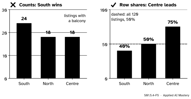
Wrong beside right. South has the most balconies because it has the most listings; per listing, Centre has the most.
“South has the most balconies, so a South flat is the most likely to have one.”
South has 24 balconies because it has 60 listings, half of all of them. Compare rows by their conditional proportions, never by raw counts: South 40 percent, Centre 75 percent.
“75 percent of Centre’s listings have a balcony, so 75 percent of balconies are in Centre.”
These divide the same count, 18, by different totals: Centre’s 24 listings, or all 60 balconies. The second is 30 percent. Say “of the …”, and name the total you divided by.
“Centre’s mean rent is 17, so Centre flats rent for about 17.”
The group has three flats and one is the penthouse; its median is 12. With small or skewed groups, give the size and the median with every mean. A model that learns a district’s typical rent from these three flats learns the penthouse’s pull along with it.
Check yourself
Recall
1. Give the mean and median rent of each district in the flats table.
Show answer
South: mean 5, median 4. North: mean 8, median 7. Centre: mean 17, median 12. Each group has three flats.
2. What did the two clumps of iris petal lengths turn out to be?
Show answer
Species: the small clump (1.0 to 1.9 cm) is setosa, and the large clump is versicolor and virginica, which overlap.
3. Define the joint, marginal and conditional proportions of a two-way table.
Show answer
Joint: a cell count over the grand total. Marginal: a row or column total over the grand total. Conditional: a cell count over its row total (or over its column total).
4. In the 120 listings, what share of Centre’s listings have a balcony, and what share of the balcony listings are in Centre?
Show answer
75 percent (18 of 24), and 30 percent (18 of 60).
5. When are two categorical columns not associated in a table?
Show answer
When every row has the same conditional proportions; then each equals the column’s marginal proportion.
Exercises
1.★ From the district-by-rating table, find the share of South’s flats rated C and the share of C-rated flats that are in South.
Show solution
South has 3 flats, 2 of them rated C (F6 and F8): \({2 / 3} = 66.7\) percent. There are 4 C-rated flats, 2 of them in South: \({2 / 4} = 50.0\) percent. Same count, different totals.
2.★★ Keep each district’s balcony share (40, 50 and 75 percent) but suppose the listings were split evenly, 40 per district. What share of all 120 would have a balcony? Why does it differ from 50 percent?
Show solution
The overall share is the weighted mean of the row shares, now with weights one third each:
That is 55 percent: 16, 20 and 30 balconies, 66 of 120. It is higher because Centre, the district with the highest share, now carries a third of the weight instead of a fifth. A change in the mix of groups alone moves an overall proportion, the seed of Simpson’s paradox in S01.7.
3.★★★ Prove that unless all rows of a two-way table have the same conditional proportion for column \(k\), at least one row lies above the marginal proportion \({n_{\cdot k} / n}\) and at least one below it.
Show solution
Write \(p_g = {n_{gk} / n_{g\cdot}}\) and \(w_g = {n_{g\cdot} / n}\). The weights are positive and add to \(1\), and the identity of the formal section says \({n_{\cdot k} / n} = {\sum_g w_g\, p_g}\). Suppose no row lay below the margin \(m = {\sum_g w_g p_g}\), so \({p_g \ge m}\) for every \(g\). Then
\[
\sum_g w_g\,(p_g - m) = m - m = 0 ,
\]
a sum of terms that are all \(0\) or more, each with a positive weight. It can be \(0\) only if every \({p_g - m} = 0\), so all rows would be equal. So if the rows are not all equal, some row lies below \(m\); the same argument with \(p_g \le m\) shows some row lies above it.
Summary card
Compare groups side by side, and compare rows by their proportions, not their counts.
S01.5.4-F1
One strip per group, sizes stated.
Number by category. Group sizes, means, medians; side-by-side boxplots when groups are large.
Two-way table. Counts \(n_{gk}\) with row and column totals.
Proportions. Joint over \(n\), marginal from the totals, conditional within one row or column.
Association. Rows with different conditional proportions; the margin is their weighted mean.
Sources and next steps
Sources. Each was opened and checked against this lesson on 12 November 2026.
David Diez, Mine Cetinkaya-Rundel and Christopher Barr, OpenIntro Statistics, fourth edition (free PDF). Section 2.1, examining numerical data, covers box plots; Section 2.2, considering categorical data, covers table proportions, bar plots and mosaic plots.
pandas developers, pandas.crosstab, pandas 3.1. The normalize argument divides by the sum of all values (‘all’ or True), of each row (‘index’) or of each column (‘columns’); margins adds row and column totals.
scikit-learn developers, sklearn.datasets.load_iris, scikit-learn 1.9. Three classes of 50 flowers, 150 in all, four measurements each, loaded as a data frame with as_frame=True.
Next. S01.6 turns to missing values, and S01.7.1 uses the conditional proportions of this lesson to show a comparison that reverses when the groups are pooled.