Plot two columns against each other and read the cloud for direction, form, strength and unusual points. Then measure how they move together with the covariance: a sum of signed rectangles, worked by hand on five points and on the nine flats.
Read a scatter plot for direction, form, strength and unusual points.
Compute a sample covariance by hand as the sum of products of deviations divided by n - 1.
Explain the sign of each product from the quadrant its point sits in, and picture it as a signed rectangle.
Show that changing x to ax multiplies the covariance by a, and say why its size alone is hard to read.
In review. The maths and code on this page are checked by automated tests on every change, but an independent reader has not signed it off yet. Spot a mistake or a confusing step? Tell us.
The question
Larger flats cost more. Everyone believes it, but how would you check it in a table of nine flats, and how would you put a number on “more”? Every model in machine learning learns from columns that move together, a feature and a target, so the first thing to look at in a new table is which columns move with which, and how.
Intuition
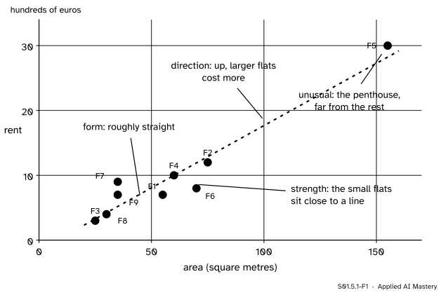
Take two numerical columns of the same table and give every row one dot: the first column sets how far right the dot sits, the second how high. The result is a scatter plot. Each dot is one row, here one flat of the course’s invented flats table, with its area across and its rent up.
S01.5.1-F1
The nine flats, area against rent. Read four things from any scatter plot: its direction, its form, its strength and any unusual points.
Four questions turn a cloud of dots into a description.
Direction. Do the dots rise from left to right, fall, or neither? Here they rise: larger flats tend to cost more.
Form. Do they follow a straight path, a curve, or separate clumps? Here, roughly a straight path.
Strength. How closely do they keep to that path? The eight ordinary flats keep fairly close.
Unusual points. Is any dot far from the rest? F5, the penthouse, sits on its own at 155 square metres and 30 hundred euros.
The picture comes first, always. The number this lesson builds, the covariance, answers only the first question, and it can be pulled about by the fourth.
Build it up
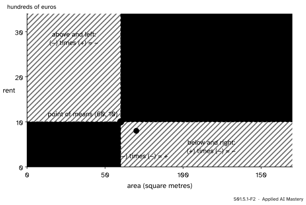
Step 1. Find the centre of the cloud. The mean area is \(\bar{x} = 60\) and the mean rent is \(\bar{y} = 10\). The point \({(60, 10)}\) is the point of means. Draw a vertical and a horizontal line through it.
Step 2. Read each flat against the centre. The two lines cut the plane into four quadrants. A flat in the upper right is larger than average and dearer than average: both of its deviations, \({x_i - \bar{x}}\) and \({y_i - \bar{y}}\), are positive, so their product is positive. A flat in the lower left is smaller and cheaper, two negatives, and the product is again positive. In the other two quadrants one deviation is positive and the other negative, so the product is negative.
S01.5.1-F2
The point of means splits the plane into four quadrants. Points that rise together land in the positive quadrants; points that go against the trend land in the negative ones.
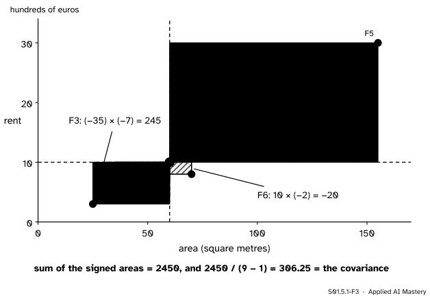
Step 3. Turn each product into a shape. The product \({(x_i - \bar{x})(y_i - \bar{y})}\) is the area of a rectangle with one corner at the point of means and the opposite corner at the flat. Give it a sign: positive in the rising quadrants, negative in the others.
S01.5.1-F3
Each flat contributes a signed rectangle. Their total, divided by \(n - 1\), is the covariance. The penthouse alone supplies 1900 of the 2450.
Step 4. Add the rectangles up and average. The signed areas add to 2450. Dividing by \({n - 1} = 8\), as for the variance in S01.3.3, gives 306.25. That number is the covariance of area and rent. It is positive because the positive rectangles outweigh the negative one.
The formal statement
NoteDefinition: sample covariance
For \(n\) rows with values \({x_1, \dots, x_n}\) in one column and \({y_1, \dots, y_n}\) in another, the covariance of \(x\) and \(y\) is
The deviations are the ones of S01.3.3, and the divisor is the same \(n - 1\). Two facts follow straight from the formula.
Its sign is the direction. Mostly positive products give \({s_{xy} > 0}\): the columns rise together. Mostly negative ones give \({s_{xy} < 0}\). When they cancel, \(s_{xy}\) is near \(0\).
A column’s covariance with itself is its variance. Put \(y = x\) and every product becomes a square: \(s_{xx} = s_x^2\).
How a change of unit acts on it. Suppose \(x\) is recorded in a new unit, \(u_i = {a x_i + b}\), with \(a\) and \(b\) fixed numbers. The mean moves the same way:
\[
\begin{aligned}
\bar{u} &= \frac{1}{n}\sum_{i=1}^{n} (a x_i + b) \\
&= a\,\frac{1}{n}\sum_{i=1}^{n} x_i + \frac{1}{n}\, n b \\
&= a\bar{x} + b .
\end{aligned}
\]
So each deviation of \(u\) is \(a\) times the deviation of \(x\), because the \(b\) cancels:
\[
\begin{aligned}
u_i - \bar{u} &= (a x_i + b) - (a\bar{x} + b) \\
&= a\,(x_i - \bar{x}) .
\end{aligned}
\]
Put that into the definition and take the common factor \(a\) outside the sum:
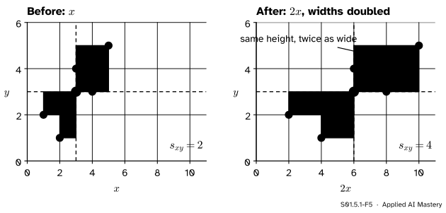
Shifting \(x\) leaves the covariance alone, and rescaling multiplies it by \(a\). In the picture, a shift moves the whole cloud and its centre together, so no rectangle changes; a stretch by \(a\) makes every rectangle \(a\) times as wide.
S01.5.1-F5
Multiplying \(x\) by \(2\) doubles every rectangle’s width and leaves its height, so the covariance doubles. Nothing about how the points move together has changed.
That is the trouble with covariance. Record rent in euros instead of hundreds of euros, \(a = 100\), and the covariance of area and rent jumps from 306.25 to 30,625 while the flats stay exactly as they were. Its units are the product of the two columns’ units, here square metres times hundreds of euros, so its size cannot be compared across tables. The next lesson divides that unit away.
Worked example
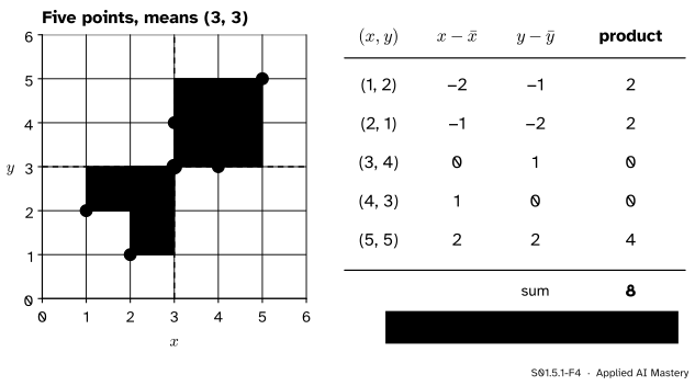
The five points. The course’s five points are \(x = 1, 2, 3, 4, 5\) and \(y = 2, 1, 4, 3, 5\). Both means are \(3\).
S01.5.1-F4
The covariance of the five points, as rectangles and as a table: products \(2, 2, 0, 0, 4\), sum \(8\), covariance \(2\).
Work row by row. The deviations of \(x\) are \(-2, -1, 0, 1, 2\) and those of \(y\) are \(-1, -2, 1, 0, 2\). Multiply in pairs:
Divide by \({n - 1} = 4\): \(s_{xy} = 2\). Two points, \((3, 4)\) and \((4, 3)\), sit on a line through the centre, so one of their deviations is \(0\) and they add nothing, whichever way they lean.
The nine flats. The same steps give the rectangles drawn in Build it up. Two of them are worth checking by hand. The penthouse has deviations \({155 - 60} = 95\) and \({30 - 10} = 20\), so its product is \({95 \times 20} = 1900\). F6 has \({70 - 60} = 10\) and \({8 - 10} = -2\), so its product is \(-20\). All nine products are \(15, 30, 245, 0, 1900, -20, 25, 180, 75\); they add to \(2450\), and \({2450 / 8} = 306.25\). The penthouse supplies 78 percent of that total on its own, a first warning that one point can make a relationship look stronger than the rest of the data say. S01.5.3 takes that warning up.
Code
From scratch first, with lists and a loop, so that every step is visible.
area = [55, 75, 25, 60, 155, 70, 35, 30, 35] # the flats table (invented), square metresrent = [7, 12, 3, 10, 30, 8, 9, 4, 7] # hundreds of euros a monthdef mean(values):returnsum(values) /len(values)def covariance(x, y): x_bar, y_bar = mean(x), mean(y) products = [(a - x_bar) * (b - y_bar) for a, b inzip(x, y)]returnsum(products) / (len(x) -1), productscov_flats, products = covariance(area, rent)print("products:", products)print("covariance of area and rent:", cov_flats)print("five points:", covariance([1, 2, 3, 4, 5], [2, 1, 4, 3, 5])[0])print("penthouse's share of the sum:", round(products[4] /sum(products), 3))
products: [15.0, 30.0, 245.0, 0.0, 1900.0, -20.0, 25.0, 180.0, 75.0]
covariance of area and rent: 306.25
five points: 2.0
penthouse's share of the sum: 0.776
numpy.cov returns a 2 by 2 covariance matrix: the two variances on the diagonal and the covariance off it. Its default divisor is \(n - 1\). pandas computes the same table for every pair of columns with DataFrame.cov.
import numpy as npimport pandas as pdmatrix = np.cov(area, rent)print(matrix)print("rent in euros:", np.cov(area, [100* r for r in rent])[0, 1])print(pd.DataFrame({"area": area, "rent": rent}).cov())
[[1593.75  306.25]
 [ 306.25   64.  ]]
rent in euros: 30625.0
         area    rent
area  1593.75  306.25
rent   306.25   64.00
The diagonal holds the variance of area, \(1593.75\), and the variance of rent, \(64\) (the standard deviation 8 of S01.3.3, squared). The scatter plot itself would be one line of Matplotlib, ax.scatter(area, rent); the course draws its pictures as figures instead.
Explore
This module’s interactive, the Anscombe explorer, lives in lesson S01.5.3. There you can drag any point of a scatter plot and watch the means, the standard deviations, the trend line and Pearson’s \(r\) (the covariance rescaled, from the next lesson) change. Drag a point into one of the negative quadrants: its product of deviations turns negative, and \(r\) falls.
Pitfalls
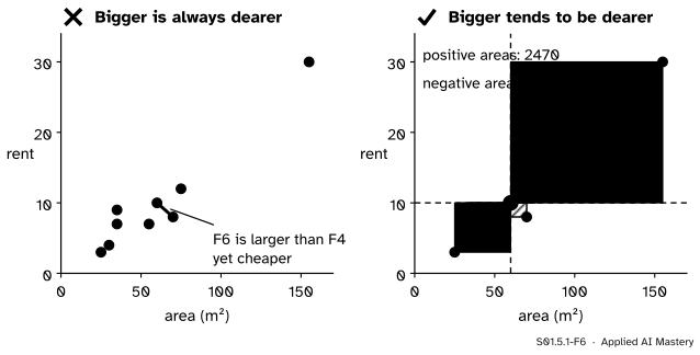
S01.5.1-F6
Wrong beside right. A positive covariance does not say that every larger flat is dearer; it says that the rising pairs outweigh the falling ones.
“The covariance is positive, so every larger flat costs more.”
Covariance is a sum over all rows, a statement about the tendency of the cloud. F6 is larger than F4 and cheaper. Single pairs can go against a positive covariance, and a few large rectangles can outweigh many small ones.
“30,625 is a huge covariance, so the link is strong.”
The size of a covariance carries the units of both columns. The same nine flats give 306.25 with rent in hundreds of euros and 30,625 with rent in euros. Only its sign can be read on its own; the correlation of the next lesson can be read on any scale.
“Covariance near zero means the columns are unrelated.”
It means the positive and negative rectangles cancel. A curve that falls and then rises can do exactly that while one column fixes the other completely, as S01.5.3 shows with \(y = x^2\). Look at the scatter plot before trusting any summary.
Check yourself
Recall
1. Name the four things to read from a scatter plot.
Show answer
Its direction (up, down or neither), its form (straight, curved, clumps), its strength (how close the points keep to that form) and any unusual points.
2. A point lies above and to the left of the point of means. What is the sign of its product of deviations?
Show answer
Negative: its \(x\)-deviation is negative and its \(y\)-deviation positive.
3. Write the definition of the sample covariance.
Show answer
The sum of the products of deviations, divided by \(n - 1\):
4. What is the covariance of a column with itself?
Show answer
Its variance, \(s_{xx} = s_x^2\), because each product becomes a square.
5. What happens to \(s_{xy}\) when every \(x\) is changed to \({a x + b}\)?
Show answer
It becomes \({a\,s_{xy}}\). The shift \(b\) cancels in every deviation; the factor \(a\) multiplies every product.
Exercises
1.★ Compute the covariance of \(x = 2, 4, 6\) and \(y = 5, 3, 1\) by hand, and say what its sign tells you.
Show solution
The means are \(\bar{x} = 4\) and \(\bar{y} = 3\). The deviations are \(-2, 0, 2\) and \(2, 0, -2\), so the products are \(-4, 0, -4\), which add to \(-8\). Dividing by \({n - 1} = 2\) gives \(s_{xy} = -4\). It is negative: as \(x\) rises, \(y\) falls. (Here the points lie exactly on a falling line.)
2.★★ The flats’ covariance of area and rent is 306.25 in square metres and hundreds of euros. One square metre is about 10.764 square feet. What is the covariance with area in square feet and rent in euros? Use the rule for a change of unit twice.
Show solution
Area in square feet is \(u = {10.764\,x}\), which multiplies the covariance by \(10.764\). Rent in euros is \(v = {100\,y}\), which multiplies it by \(100\). The rule applies to each column in turn, because covariance treats its two columns alike. So the new covariance is \({306.25 \times 10.764 \times 100}\), about \(329{,}648\). The flats did not change; only the units did.
3.★★★ Show that the products of deviations can be computed without the mean of \(y\), that is, prove
The deviations from the mean sum to zero (S01.3.1), so the last sum is \(0\) and the first term is all that is left. On the five points the deviations of \(x\) are \(-2, -1, 0, 1, 2\) and the \(y\) values are \(2, 1, 4, 3, 5\), so the sum is \({-4 - 1 + 0 + 3 + 10} = 8\), as in the worked example.
Summary card
Plot first; then let the signed rectangles say which way the columns move together.
S01.5.1-F3
Covariance: signed rectangles, averaged.
Scatter plot. One dot per row; read direction, form, strength, unusual points.
Covariance.\(s_{xy}\) is the sum of products of deviations over \(n - 1\); five points: \(2\).
Sign. Positive when the columns rise together, negative when one falls as the other rises.
Units.\(x \to {ax + b}\) gives \(s_{xy} \to {a\,s_{xy}}\), so only the sign reads on its own.
Sources and next steps
Sources. Each was opened and checked against this lesson on 12 November 2026.
NumPy developers, numpy.cov, NumPy 2.5 reference. For two one-dimensional arrays it returns the 2 by 2 covariance matrix, and its default normalisation divides by \(N - 1\).
Next.S01.5.2 Correlation divides the covariance by both standard deviations and gets a number that is the same in every unit.