Deleting incomplete rows is the default of most tools, and it costs more than it looks: ten columns with a tenth of their values missing keep only 35 percent of the rows. Derive that cost, see when deletion is a fair sample and when it is selection, and compare listwise, pairwise and column deletion.
Derive the share of rows that survive listwise deletion, (1 - p) to the power k, and evaluate it.
Explain why the complete rows are a simple random sample of the rows only under MCAR, and are a selection otherwise.
Compare listwise and pairwise deletion, and find the rows that each statistic of a pairwise analysis rests on.
Decide between dropping rows and dropping a column, and record how many rows each cleaning step removes.
In review. The maths and code on this page are checked by automated tests on every change, but an independent reader has not signed it off yet. Spot a mistake or a confusing step? Tell us.
The question
A table has ten columns, and each is missing only one value in ten. That sounds healthy. Then a model, like most tools, quietly throws away every row with a hole, and two thirds of the table are gone. Why do so few rows survive, and when are the survivors still a fair picture of the rest?
From the last lesson
1. Dear flats write “price on request”. Which mechanism is this, and why can weighting by district not repair it?
Show answer
MNAR: the chance of a hole depends on the hidden rent itself. Inside each district the dear rents are the ones lost, so each district’s mean of the rents seen is too low, and weights cannot fix a biased group mean.
2. Under MAR, what kind of sample are the values seen inside one group?
Show answer
A simple random sample of that group, because inside the group every row has the same chance of a hole.
Intuition
The quickest repair for holes is to delete them. Listwise deletion (also called complete-case analysis) keeps only the rows with no hole in any column. It is what some tools do without being asked: a regression in R, for one, drops every incomplete row before it fits.
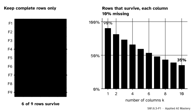
On the flats table with its five holes (S01.6.1), listwise deletion strikes out F4, F7 and F9 and keeps six rows. That is the visible cost. The hidden cost grows with the number of columns, because a row needs every one of its cells to survive.
S01.6.3-F1
Listwise deletion. Left: on the flats table, three rows go and six survive. Right: when each column misses \(10\%\) of its values, the share of complete rows falls from \(90\%\) with one column to \(35\%\) with ten.
And a second question matters more than the count: which rows survive? The answer comes straight from the last lesson. The complete rows are the rows that the missingness mechanism spared, so they are a fair sample only if the mechanism spares rows by chance.
Build it up
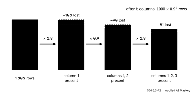
Step 1. One column. Take \(1{,}000\) rows and a column with \(10\%\) of its values missing. Then \(900\) rows have that value.
Step 2. A second column. Suppose the holes of column 2 have nothing to do with those of column 1: among any group of rows, column 2 is missing in about \(10\%\). Then of the \(900\) rows that have column 1, \(10\%\) lose column 2, and \({900 \times 0.9} = 810\) have both.
Step 3. Keep going. Each new column keeps \(0.9\) of the rows still standing: \({810 \times 0.9} = 729\) after three columns, and after \(k\) columns \({1000 \times 0.9^k}\).
S01.6.3-F2
A share of a share. Each column keeps \(90\%\) of the rows that are still complete, so the losses compound like interest: \(1{,}000\), then \(900\), \(810\), \(729\).
Step 4. Who survives? Under MCAR every row has the same chance of being complete, so the complete rows are a simple random sample of all rows (S01.2.1): fewer, and fair. Under MAR or MNAR, rows with holes differ from rows without, so deletion keeps a selection of the rows, the selection of S01.2.4 carried out by the analyst. In the city of the last lesson, dropping the rows whose rent was hidden left a mean rent of \(6.70\) under MAR and \(6.66\) under MNAR, against \(8.3\).
The formal statement
NoteResult: the share of complete rows
If each of \(k\) columns misses a share \(p\) of its values, and the holes in one column are independent of those in the others, then the share of rows with no hole is
\[
(1 - p)^k .
\]
Derivation. Write \(S_j\) for the share of rows that are complete in the first \(j\) columns. With no columns, every row counts, so \(S_0 = 1\). A row is complete in the first \(j\) columns when it is complete in the first \({j - 1}\) and has column \(j\). Independence says that column \(j\) is present in a share \({1 - p}\) of any group of rows, including the group complete so far, so
With \(p = 0.1\) and \(k = 10\), \(S_{10} = 0.9^{10} = 0.349\): about \(35\%\) of the rows survive. If the columns have different shares \({p_1, \dots, p_k}\), the same steps give the product \({(1 - p_1)(1 - p_2) \cdots (1 - p_k)}\).
Three ways to delete.
Listwise deletion keeps the complete rows and uses them for everything. Every statistic rests on the same rows, and under MCAR they are a fair sample; otherwise they are a selection.
Pairwise deletion (or available-case analysis) lets each statistic use every row that has the columns it needs. The mean of rent uses every row with a rent; the correlation of area with rent uses every row with both. Nothing is wasted, but each number rests on a different sample, so two statistics may describe different sets of flats. DataFrame.corr works this way and says so only in its documentation.
Column deletion drops a column that is mostly holes, so that its holes no longer remove rows.
S01.6.3-F4
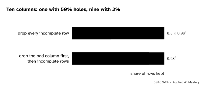
One bad column can halve a table. With it, listwise deletion keeps \({0.5 \times 0.98^{9}} = 41.7\%\) of the rows; without it, \(0.98^{9} = 83.4\%\). Whether the column can be spared is a question about the analysis, not about the numbers.
Worked example
The flats table with its five holes: listwise against pairwise deletion. The stand-ins have been turned into NaN, so built misses F9, area misses F4 and F7, and rent misses F4 and F7.
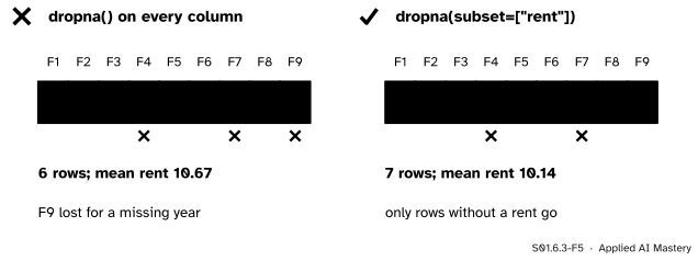
Listwise. Rows F4, F7 and F9 have holes, so six rows remain: F1, F2, F3, F5, F6 and F8. Their rents are \(7, 12, 3, 30, 8, 4\), with sum \(64\) and mean \({64/6} = 10.67\). Notice that F9 was thrown away although its rent, \(7\), was known: its only fault was a missing year.
Pairwise. Each statistic takes the rows it can use.
S01.6.3-F3
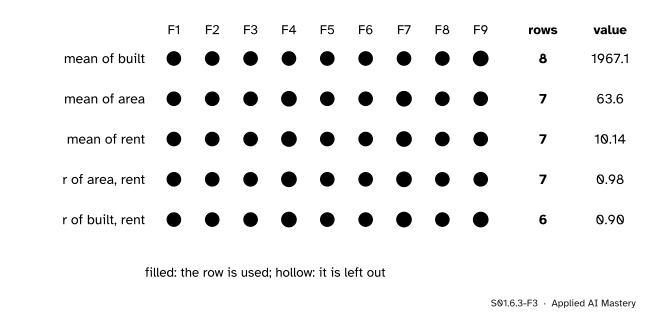
Pairwise deletion. Each line is one statistic, each dot one flat. The five numbers rest on three different sets of rows: \(8\), \(7\) and \(6\) flats.
The mean of rent now uses seven rows: \({71/7} = 10.14\). The correlation of area with rent uses the same seven and is \(0.98\), while the correlation of year built with rent uses only six and is \(0.90\). A table of correlations built this way mixes samples, and van Buuren notes that such a table need not even hang together as a correlation table of any one set of rows.
A cleaning log. Every deletion is a decision, so write it down:
step
rows before
rows after
stand-ins to NaN
9
9
drop rows with no rent
9
7
drop rows with no area
7
7
The second line removed F4 and F7; the third removed nothing more, because the same two rows had lost both values.
Code
From scratch, first the filter and then a check of \({(1 - p)^k}\) by simulation.
import mathnan =float("nan")rows = {"F1": (1964, 55, 7), "F2": (1996, 75, 12), "F3": (1932, 25, 3), "F4": (1988, nan, nan),"F5": (2019, 155, 30), "F6": (1975, 70, 8), "F7": (1905, nan, nan), "F8": (1958, 30, 4),"F9": (nan, 35, 7)} # built, area, rent; stand-ins already NaNcomplete = {k: v for k, v in rows.items() ifnotany(math.isnan(x) for x in v)}rents = [v[2] for v in complete.values()]print("complete rows:", list(complete), " mean rent", round(sum(rents) /len(rents), 2))with_rent = [v[2] for v in rows.values() ifnot math.isnan(v[2])]print("rows with a rent:", len(with_rent), " mean rent", round(sum(with_rent) /len(with_rent), 2))print("formula: 0.9 ** 10 =", round(0.9**10, 4), " 0.5 * 0.98 ** 9 =", round(0.5*0.98**9, 4))
complete rows: ['F1', 'F2', 'F3', 'F5', 'F6', 'F8']  mean rent 10.67
rows with a rent: 7  mean rent 10.14
formula: 0.9 ** 10 = 0.3487   0.5 * 0.98 ** 9 = 0.4169
import numpy as nprng = np.random.default_rng(0)holes = rng.random((100_000, 10)) <0.1# each cell missing with chance 0.1share_complete = (~holes.any(axis=1)).mean()print("simulated share of complete rows:", round(share_complete, 3), " formula:", round(0.9**10, 3))
simulated share of complete rows: 0.347 formula: 0.349
Now pandas. dropna drops incomplete rows; subset limits the columns it looks at, thresh keeps rows with at least that many values, and axis=1 drops columns instead. corr computes each correlation on the rows that have both columns.
[('listwise', 9, 6), ('rows with a rent', 9, 7), ('at least 5 values', 9, 7)]
mean rent, listwise 10.67  subset 10.14
columns kept by dropna(axis=1): ['district', 'rating', 'rooms']
       built  area  rent
built   1.00  0.92  0.90
area    0.92  1.00  0.98
rent    0.90  0.98  1.00
The correlations printed by corr rest on different rows: seven for area with rent, six for each pair that involves the year built. Nothing in the printed table tells you so.
Explore
Go back to the missingness machine in lesson S01.6.2 and choose Drop those rows. Lose rents at random and press New draw: the mean wobbles but does not lean. Then lose high rents: almost every draw gives a mean that is too low, and the lean grows as you lose more.
Pitfalls
S01.6.3-F5
Wrong beside right. To average the rents, drop the rows without a rent and nothing else. Dropping every incomplete row also throws away F9’s known rent.
“My model trained without errors, so the data were complete.”
Some fitting functions, R’s regression among them, drop incomplete rows without a word; many scikit-learn models stop with an error instead. Count the rows that went in and the rows that came out. In machine learning the same deletion at prediction time is worse: a new row with one hole gets no prediction at all, and the model was never tested on rows like it.
“Deleting holes is neutral; it just shrinks the sample.”
Only under MCAR. Otherwise the complete rows are a selection, and every summary leans with them: in the city, the rows with a rent left under MNAR averaged \(6.66\) against a true \(8.3\).
“Pairwise deletion is always better, because it uses more data.”
It uses more rows for each number, but the numbers no longer describe one set of flats. Two means from different rows cannot be compared as if they came from the same flats, and a table of pairwise correlations need not be consistent. Under MCAR both methods are fair; under MAR or MNAR both lean.
Check yourself
Recall
1. What share of rows survives listwise deletion when each of \(k\) independent columns misses a share \(p\)?
Show answer
\({(1 - p)^k}\). For example, \(0.9^{10} = 0.349\) for ten columns at \(10\%\).
2. Under which mechanism are the complete rows a simple random sample of all rows?
Show answer
MCAR. Under MAR or MNAR they are a selection.
3. What is the difference between listwise and pairwise deletion?
Show answer
Listwise keeps only the complete rows and uses them for every statistic. Pairwise lets each statistic use every row that has the columns it needs, so different statistics rest on different rows.
4. On the flats table with holes, why does listwise deletion give a mean rent of \(10.67\) while dropna(subset=["rent"]) gives \(10.14\)?
Show answer
Listwise deletion also drops F9 for its missing year, although its rent of \(7\) is known. With F9 the seven rents average \({71/7} = 10.14\); without it, the six average \({64/6} = 10.67\).
5. What does dropna(thresh=5) keep?
Show answer
The rows with at least five values that are not missing.
Exercises
1.★ A table has \(20\) columns, each missing \(5\%\) of its values independently. What share of rows is complete? How many of \(2{,}000\) rows is that?
Show solution
\(0.95^{20} = 0.3585\), so about \(35.8\%\). Of \(2{,}000\) rows that is \({2000 \times 0.3585} = 716.97\), about \(717\) rows.
2.★★ You want at least half of the rows to survive listwise deletion with \(k = 10\) independent columns. What is the largest share \(p\) of holes per column you can allow?
Show solution
Solve \({(1 - p)^{10} \ge 0.5}\). Take the tenth root of both sides: \({1 - p \ge 0.5^{1/10}}\). Then \({0.5^{1/10}} = 0.933\) (with logarithms: \({\ln 0.5 / 10} = {-0.0693}\), and \({e^{-0.0693}} = 0.933\)), so \({p \le 0.067}\): at most about \(6.7\%\) per column.
3.★★★ In the city of lesson S01.6.2, rents are hidden by district (MAR). You drop the rows without a rent and then compute each district’s mean rent from the rows left. Are these three means fair? Is the overall mean of the rows left fair? Explain with the mechanisms.
Show solution
The district means are fair: under MAR by district, the rents seen inside each district are a simple random sample of that district, so each district mean has no lean. The overall mean of the rows left is not: Centre lost \(80\%\) of its rents and the other districts \(10\%\), so Centre is under-represented among the rows left, and the plain mean leans low: on average \(6.70\) against \(8.3\). Weighting the three fair district means by the shares \(0.5\), \(0.3\) and \(0.2\) repairs it.
Summary card
Deleting is cheap to type and expensive to do.
S01.6.3-F1
Rows vanish as columns add up.
Survival:\({(1 - p)^k}\) of the rows are complete; \(0.9^{10} = 0.35\).
Fair only under MCAR; under MAR and MNAR deletion is selection.
Listwise: one set of rows. Pairwise: each statistic its own rows.
pandas:dropna(subset=..., thresh=..., axis=...); corr is pairwise.
Sources and next steps
Sources. Each was opened and checked against this lesson on 12 November 2026.
Stef van Buuren, Flexible Imputation of Missing Data, second edition, Sections 1.3.1 and 1.3.2. Listwise deletion gives unbiased estimates of means, variances and regression weights under MCAR, can severely bias them otherwise, and often loses a large part of the sample; pairwise deletion uses all the data for each statistic, and its covariance matrix may fail to be positive definite.
Andrew Gelman and Jennifer Hill, Data Analysis Using Regression and Multilevel/Hierarchical Models, Section 25.2. That R drops incomplete rows automatically in classical regressions; the two problems of complete-case analysis (bias when the incomplete cases differ, and few complete cases when there are many variables), and available-case analysis, whose summaries rest on different subsets and so may not be consistent with each other.
pandas developers, DataFrame.dropna and DataFrame.corr, pandas 3.1.1 API reference. The parameters axis, how, thresh and subset, and the note that correlations are computed using pairwise complete observations.
Next.S01.6.4 Filling in keeps every row by filling the holes instead, and prices that too.