Draw inside each district and weight the district means by their shares of the city: the course’s first weighted mean. See why stratifying cuts the scatter, what whole buildings and every 25th listing save and risk, and how a stratified data split uses the same idea.
Derive the population mean as the stratum means weighted by the stratum shares, and compute it for the city.
Compute a stratified estimate from a sample, and explain why the plain mean of an equal-allocation sample is biased.
Explain why stratified sampling scatters less than a simple random sample of the same size when the strata differ.
Describe cluster and systematic sampling, with what each saves and what each risks.
Draw a stratified sample with pandas and weight it with numpy.average, and stratify a train-test split with scikit-learn.
In review. The maths and code on this page are checked by automated tests on every change, but an independent reader has not signed it off yet. Spot a mistake or a confusing step? Tell us.
The question
Each district’s three flats in the table have exactly that district’s mean rent: 5 in South, 8 in North and 17 in Centre. Yet the nine flats average 10, while the city averages 8.3. Nothing in the table is wrong. So where does the gap come from, and how do you turn the table into the right answer?
From the last lesson
1. A sample is drawn by lot from a frame whose mean is \(\mu_F\). What is its bias, and how does it change with \(n\)?
Show answer
\(\mu_F - \mu\), the same at every sample size.
2. In the city simulation, what happened to the scatter of simple random samples each time \(n\) was multiplied by four?
Show answer
It about halved: 2.12, 1.06 and 0.50 at \(n = 4\), 16 and 64.
Intuition
The city is not one crowd of 500 flats. It is three districts that differ a great deal: Centre’s flats cost more than three times South’s. A stratum (plural strata) is such a group, and a stratified sample is drawn separately, by lot, inside each stratum.
S01.2.3-F1
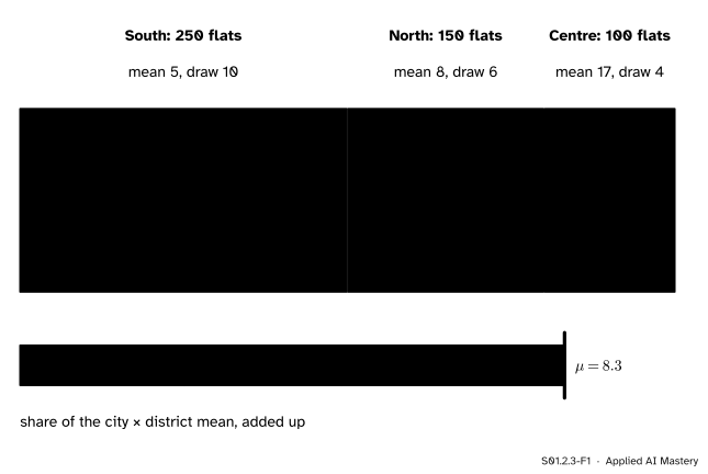
A stratified sample of 20 draws 10, 6 and 4 flats by lot inside South, North and Centre. Below, the city’s mean built from its parts: each district adds its share of the city times its mean.
Two ideas sit in the picture. The top half is the sampling: every district is guaranteed its right number of flats, so a sample can never come back with no Centre flats, or with mostly Centre flats, by bad luck. The bottom half is the arithmetic: a mean of the whole is a weighted mean of the means of the parts, each weighted by its share. That second idea answers the question of the hook.
Build it up
Step 1. Totals add. The city’s total rent is South’s total plus North’s plus Centre’s. A district’s total is its number of flats times its mean: \({250 \times 5} = 1250\), \({150 \times 8} = 1200\) and \({100 \times 17} = 1700\), which add to 4150.
Step 2. Divide by the count. The city’s mean is \(4150 / 500 = 8.3\). Splitting the division over the three totals gives the same number in a more useful form:
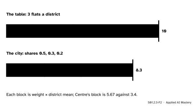
The same three district means, averaged with two sets of weights. Giving Centre a third of the weight when it holds a fifth of the flats lifts the mean from 8.3 to 10.
That is the gap of the hook. The table’s means are right; its mix is wrong. Centre is a fifth of the city but a third of the table.
Step 4. Weight the sample the same way. If the district means of a sample stand in for the districts’ true means, weighting them with the city’s shares gives an estimate of \(\ctruth{\mu}\). That is the stratified estimate.
The formal statement
NoteStratified sampling
A population of \(N\) units is split into strata \(g = 1, \dots, G\). Stratum \(g\) holds \(N_g\) units with mean \(\mu_g\), and its share is \(\cparam{W_g} = N_g / N\). A stratified sample draws a simple random sample of \(n_g\) units inside each stratum, separately. With \(\bar{x}_g\) the mean of the units drawn from stratum \(g\), the stratified estimate of \(\mu\) is
The population mean is a weighted mean. Every unit belongs to exactly one stratum, so the population total is the sum of the stratum totals, and stratum \(g\)’s total is \(N_g \mu_g\). Divide by \(N\):
The shares add to \(\sum_g N_g / N = N / N = 1\), as weights of a mean must.
The stratified estimate is unbiased. Inside stratum \(g\) the draw is a simple random sample, so over all its possible samples \(\bar{x}_g\) averages exactly \(\mu_g\) (lesson S01.2.1). The strata are drawn separately, so every combination of one sample from each stratum is equally likely. Averaging \(\cparam{W_1}\bar{x}_1 + \cparam{W_2}\bar{x}_2 + \cdots\) over all those combinations averages each term on its own, because a weight is a fixed number and an average of a sum is the sum of the averages. So the centre of the stratified estimate is \(\sum_g \cparam{W_g}\, \mu_g = \ctruth{\mu}\): no bias.
Proportional allocation weighs itself. If each stratum gets its share of the sample, \(n_g = n\, W_g\), then \(W_g = n_g / n\) and
\[
\begin{aligned}
\sum_{g} \frac{n_g}{n}\, \bar{x}_g
&= \frac{1}{n} \sum_{g} n_g\, \bar{x}_g \\
&= \frac{\text{sum of all values}}{n} ,
\end{aligned}
\]
because \(n_g \bar{x}_g\) is the sum of stratum \(g\)’s values. The stratified estimate is then just the plain mean of the sample. For \(n = 20\) in the city, proportional allocation is 10, 6 and 4.
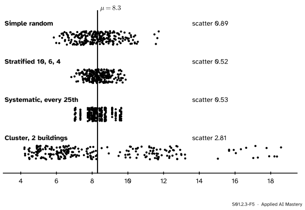
Why stratifying scatters less. The mean of a simple random sample moves for two reasons: the flats it holds inside each district vary, and so does its mix of districts. One sample of 20 might hold 2 Centre flats and the next 7, and since Centre’s rents are so much higher, the mean swings with the mix. Stratifying fixes the mix and leaves only the first reason. The more the strata differ, the more scatter it removes. The simulation shows it:
S01.2.3-F5
One thousand estimates of \(\ctruth{\mu}\) from each design, each using 20 flats of the city (250 of them drawn). All four are centred on 8.3. Stratified and systematic samples scatter little more than half as much as a simple random one; two whole buildings scatter three times as much.
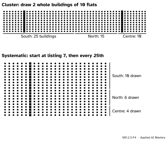
Cluster sampling. A cluster sample draws whole groups, called clusters, and keeps every unit in each. Suppose the city’s flats stand in 50 buildings of 10 neighbours each. Visiting 2 buildings is far cheaper than visiting 20 flats spread over the city. The risk is that neighbours are alike: here a building lies in one district, so two buildings tell you about at most two districts, and the estimate scatters by 2.81. Clusters work best when each is a small copy of the population.
Systematic sampling. A systematic sample takes every \(k\)-th unit of a list, from a start chosen by lot. With \(N = 500\) and \(n = 20\), \(k = 500 / 20 = 25\). There are 25 possible starts, and every flat is in exactly one of the 25 samples, so (as in lesson S01.2.1) their means average exactly \(\ctruth{\mu}\). It is easy to carry out by hand. On a list sorted by district it even acts like proportional stratification, since every run of 25 listings contributes one flat: 10 from South, 6 from North and 4 from Centre. The risk is a list with a repeating pattern: if every 25th listing were a paid “featured” slot, a systematic sample could be all featured flats.
S01.2.3-F4
Top: a cluster sample takes two whole buildings. Bottom: written in rows of 25, every 25th listing is one column, so a systematic sample of a list sorted by district takes 10, 6 and 4 flats from the three districts.
Worked example
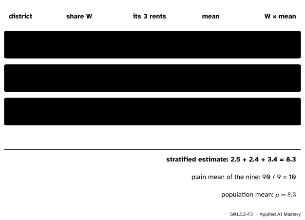
The nine flats as a stratified sample. The table drew three flats from each district. Read it as a stratified sample and weight it by the city’s shares.
S01.2.3-F3
The stratified estimate from the nine flats. Each district mean is weighted by the district’s share of the city.
South (F3, F6, F8): rents 3, 8 and 4 add to 15, so \(\bar{x}_1 = 5\), and its share is \(250 / 500 = 0.5\). North (F1, F4, F9): rents 7, 10 and 7 add to 24, so \(\bar{x}_2 = 8\), with share 0.3. Centre (F2, F5, F7): rents 12, 30 and 9 add to 51, so \(\bar{x}_3 = 17\), with share 0.2. Then
The plain mean of the nine is \(90 / 9 = 10\). Here the stratified estimate lands exactly on \(\ctruth{\mu}\) only because the invented city was built so that its district means are those of the nine flats. A real sample’s district means would miss a little, and the stratified estimate with them. The plain mean, by contrast, misses by 1.7 for a reason that has nothing to do with luck: equal allocation over-weights Centre.
Code
From scratch, a stratified draw and its estimate on the city. The city is built as in every lesson of the course.
import numpy as npimport pandas as pdrng = np.random.default_rng(0)sizes = {"South": 250, "North": 150, "Centre": 100}district_mean = {"South": 5, "North": 8, "Centre": 17}rents, district = [], []for name in ("South", "North", "Centre"): draws = rng.gamma(9.0, 1.0, sizes[name]) rents.append(draws * district_mean[name] / draws.mean()) district += [name] * sizes[name]rents, district = np.concatenate(rents), np.array(district)mu = rents.mean()share = {d: sizes[d] /len(rents) for d in sizes}print("shares:", share, " weighted mean of district means:",sum(share[d] * district_mean[d] for d in sizes))def stratified_estimate(take, rng): total =0.0for d, n_d in take.items(): drawn = rng.choice(rents[district == d], n_d, replace=False) total += share[d] * drawn.mean()return totalrng = np.random.default_rng(1)simple = np.array([rng.choice(rents, 20, replace=False).mean() for _ inrange(1000)])strat = np.array([stratified_estimate({"South": 10, "North": 6, "Centre": 4}, rng) for _ inrange(1000)])scatter =lambda v: np.abs(v - v.mean()).mean()print(f"simple random: centre {simple.mean():.2f}, scatter {scatter(simple):.2f}")print(f"stratified: centre {strat.mean():.2f}, scatter {scatter(strat):.2f}")
shares: {'South': 0.5, 'North': 0.3, 'Centre': 0.2}  weighted mean of district means: 8.3
simple random: centre 8.25, scatter 0.89
stratified:    centre 8.29, scatter 0.52
These are the first two rows of the figure. The same generator, carried on, gives the other two: a systematic sample from a start drawn by lot, and two whole buildings of ten neighbouring flats.
systematic = np.array([rents[int(rng.integers(25))::25].mean() for _ inrange(1000)])buildings = rents.reshape(50, 10) # a building is 10 neighbours in the listcluster = np.array([buildings[rng.choice(50, 2, replace=False)].mean() for _ inrange(1000)])print(f"systematic: centre {systematic.mean():.2f}, scatter {scatter(systematic):.2f}")print(f"cluster: centre {cluster.mean():.2f}, scatter {scatter(cluster):.2f}")every_start = [rents[r::25].mean() for r inrange(25)]print(f"mean over all 25 starts: {np.mean(every_start):.6f}")
systematic:    centre 8.30, scatter 0.53
cluster:       centre 8.35, scatter 2.81
mean over all 25 starts: 8.300000
Over all 25 starts the systematic means average exactly 8.3, as every flat is in exactly one of them. Now the nine flats with numpy.average, which divides the weighted sum by the sum of the weights.
pandas draws inside each group with DataFrameGroupBy.sample. With frac=0.04 each district gives 4 percent of its flats: proportional allocation for \(n = 20\).
city = pd.DataFrame({"district": district, "rent": rents})drawn = city.groupby("district").sample(frac=0.04, random_state=1)print(drawn["district"].value_counts().to_dict())
{'South': 10, 'North': 6, 'Centre': 4}
A train-test split is a sample too (ML01.2.2). Passing stratify to scikit-learn’s train_test_split keeps every group’s share in both parts, which matters most for a rare class.
The stratified test set holds exactly 50, 30 and 20 flats, a half, three tenths and a fifth of 100. The plain split’s counts depend on the seed.
Explore
This module’s interactive, the sampling bench, lives in lesson S01.2.2. Its near the corner method is the opposite of stratifying: it lets one part of the town stand for all of it.
Pitfalls
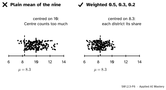
S01.2.3-F6
Wrong beside right, over 1,000 samples of three flats per district. Averaged plainly, they centre on 10; weighted by the districts’ shares of the city, on 8.3.
“A stratified sample can be averaged like any other sample.”
Only if each stratum got its share of the sample. The flats table drew three per district, so its plain mean centres on \({(5 + 8 + 17) / 3} = 10\), a bias of \(+1.7\). Weight the district means by the shares \(N_g / N\), or allocate the sample in proportion, and the bias goes.
“Two buildings of ten are as good as twenty flats drawn by lot.”
Twenty flats in two buildings are not twenty separate looks at the city, because neighbours are alike. In the simulation two buildings scatter by 2.81, three times as much as 20 flats by lot. Cluster samples save money and spend precision.
“Every k-th row is as good as a random sample.”
Only if the list has no pattern that repeats every \(k\) rows. A log written every hour and sampled every 24th row sees the same hour of every day. In machine learning, taking every 10th row of a file sorted by class or by time for a test set is the same trap.
Check yourself
Recall
1. Write the population mean in terms of the stratum means and shares.
Show answer
\(\mu = \sum_g W_g\, \mu_g\), with \(W_g = N_g / N\); for the city \({0.5 \cdot 5} + {0.3 \cdot 8} + {0.2 \cdot 17} = 8.3\).
2. Why do the nine flats average 10 when the city averages 8.3?
Show answer
They hold three flats per district, so their plain mean weights each district by a third. Centre, the dearest district, is a fifth of the city but a third of the table.
3. When does a stratified estimate need no weights?
Show answer
Under proportional allocation, \(n_g = n W_g\): then the stratified estimate equals the plain mean of the sample.
4. Why does stratifying the city reduce the scatter?
Show answer
It fixes the mix of districts in every sample, so the mean no longer swings with how many dear Centre flats happened to be drawn. Only the variation inside districts is left.
5. What does each of cluster and systematic sampling save, and what does each risk?
Show answer
Cluster sampling saves travel and cost by taking whole groups, but risks a large scatter when members of a group are alike. Systematic sampling is simple to carry out, but risks a list whose pattern repeats every \(k\) units.
Exercises
1.★ Another city has 300 flats in South with mean rent 5, 200 in North with mean 8 and 100 in Centre with mean 17. Find the shares and \(\mu\).
Show solution
\(N = 600\), so the shares are \(300/600 = 0.5\), \(200/600 = 1/3\) and \(100/600 = 1/6\). Then
2.★★ In the city a stratified sample of 50 uses proportional allocation. How many flats come from each district? A sample gives district means 5.2, 7.6 and 18.0: find the stratified estimate, and check that it equals the plain mean of the 50 rents.
Show solution
\(n_g = 50\, W_g\): 25 from South, 15 from North and 10 from Centre. The estimate is
The sums of the rents are \({25 \cdot 5.2} = 130\), \({15 \cdot 7.6} = 114\) and \({10 \cdot 18} = 180\), which add to 424, and \(424 / 50 = 8.48\). The two agree, as proportional allocation promises.
3.★★★ A sample takes three flats by lot from each district of the city and reports the plain mean of the nine. (a) Show that its centre over all possible samples is \({(\mu_1 + \mu_2 + \mu_3) / 3}\), and find its bias. (b) Which weights remove the bias?
a weighted mean with weights one third. Each \(\bar{x}_g\) is a simple random sample’s mean inside its district, so it averages \(\mu_g\), and the average of the sum is the sum of the averages. The centre is \({(5 + 8 + 17) / 3} = 10\) and the bias is \(10 - 8.3 = +1.7\).
(b) The shares \(W_g\): 0.5, 0.3 and 0.2. Then the centre is \(\sum_g W_g \mu_g = \mu\).
Summary card
Draw inside each group, then weight each group by its share.
Proportional allocation\(n_g = n W_g\): the plain mean already is the stratified estimate.
Cluster: cheap, scatters more. Systematic: simple, beware patterns in the list.
Sources and next steps
Sources. Each was opened and checked against this lesson on 12 November 2026.
David Diez, Mine Cetinkaya-Rundel and Christopher Barr, OpenIntro Statistics, 4th edition, Section 1.3.5, “Four sampling methods”: stratified sampling helps most when cases inside a stratum are similar; cluster sampling can be more economical and works best when the clusters do not look very different from one another.
Barbara Illowsky and Susan Dean, Introductory Statistics 2e, OpenStax, Section 1.2: stratified samples take a proportionate number from each stratum, and a systematic sample takes every \(n\)-th item of a list from a random start.
NumPy, numpy.average: the weighted average is sum(a * weights) / sum(weights).
pandas, DataFrameGroupBy.sample: returns a random sample of items from each group, with n or frac per group.
scikit-learn, train_test_split: with stratify, the data are split in a stratified fashion using the given labels.