Four sets of eleven points share their means, variances, correlation 0.816 and trend line, yet one is a cloud, one a curve, one a line with an outlier and one a stack. Learn why r sees only straight lines, how one point can make it, and how Spearman’s rank correlation resists.
Explain with Anscombe’s quartet why a scatter plot must come before any summary of two columns.
Show by calculation that r measures straight-line association only, using y = x squared on x = -2, …, 2.
Measure how much one point moves r, on the flats with and without the penthouse.
Compute Spearman’s rank correlation by hand as Pearson’s r on ranks, with tied values given their average rank.
In review. The maths and code on this page are checked by automated tests on every change, but an independent reader has not signed it off yet. Spot a mistake or a confusing step? Tell us.
The question
Someone hands you four data sets and a table of summaries: the same means, the same variances, the same correlation \(0.816\) and the same trend line for all four. Are the four the same? A model that sees only such summaries, or a feature screen that keeps the columns with the largest \(r\), would treat them alike. What can a correlation not see?
From the last lesson
1. Write Pearson’s \(r\) in two ways: with z-scores, and with the covariance.
Show answer
\(r\) is the sum of \({z_{x,i}\, z_{y,i}}\) divided by \(n - 1\), and it equals \({s_{xy} / (s_x s_y)}\).
2. Between which values does \(r\) lie, and when does it reach the ends?
Show answer
Between \(-1\) and \(1\). It reaches \(1\) or \(-1\) exactly when the points lie on a rising or a falling straight line.
Intuition
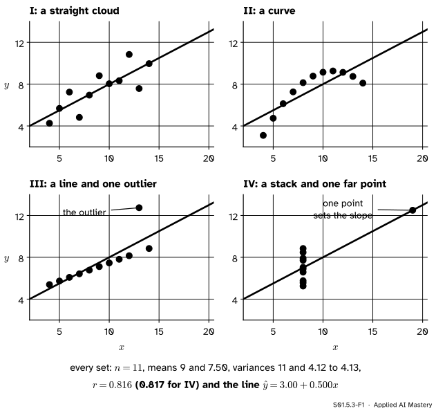
In 1973 the statistician F. J. Anscombe made up four small data sets to make one point: compute the usual summaries, and then look. Each set has eleven points. Their summaries agree to two or three decimals. Their pictures do not.
S01.5.3-F1
Anscombe’s quartet. One table of summaries fits all four; only the first looks like what the table suggests.
Set I is what \(r = 0.816\) makes you picture: a straight cloud with some scatter.
Set II is a smooth curve. A straight line is the wrong shape for it.
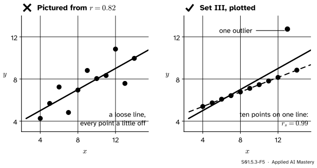
Set III is an almost perfect line with one point knocked off it. That one point drags \(r\) down from almost \(1\).
Set IV has no relationship you can see at all: ten points share one \(x\) value, and a single far point decides the slope on its own.
The rule that follows is short. Plot before you summarise. A summary is a compression, and a compression throws something away. The scatter plot shows what.
Build it up
Three facts explain the quartet.
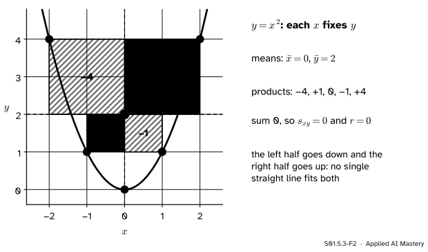
Step 1. \(r\) sees only straight lines. Take \(x = -2, -1, 0, 1, 2\) and \(y = x^2\), so \(y = 4, 1, 0, 1, 4\). Each \(y\) is fixed exactly by its \(x\); there could not be a closer relationship. Yet the signed rectangles of S01.5.1 cancel in pairs.
S01.5.3-F2
\(y = x^2\): the left half falls and the right half rises, and their rectangles cancel. The covariance is \(0\), so \(r = 0\), although \(x\) fixes \(y\) completely.
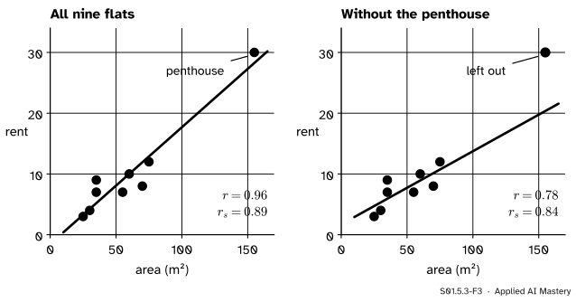
Step 2. One point can make \(r\). Go back to the flats, area against rent. With all nine, \(r = 0.96\). Leave out the penthouse and the eight ordinary flats give \(r = 0.78\). In S01.5.1 its rectangle was 78 percent of the whole sum; here it lifts a moderate correlation into a very strong one.
S01.5.3-F3
The penthouse lifts \(r\) from \(0.78\) to \(0.96\). Spearman’s \(r_s\), built in Step 3, moves only from \(0.84\) to \(0.89\).
Step 3. Ranks take the pull away. Replace each value by its rank: \(1\) for the smallest, \(2\) for the next, and so on. The penthouse’s rent of 30 becomes rank 9, one step above the next dearest, whatever its size. Correlating the ranks instead of the values is Spearman’s idea.
The formal statement
Why \(y = x^2\) gives exactly \(r = 0\). The means are \(\bar{x} = 0\) and \(\bar{y} = {(4 + 1 + 0 + 1 + 4)/5} = 2\). Since \(\bar{x} = 0\), each \(x\)-deviation is \(x_i\) itself, so the sum of products is
The covariance is \(0\) and so is \(r\). The cubes cancel because every \(x\) has a partner \(-x\). Any set of \(x\) values balanced in pairs about \(0\), with \(y = x^2\), gives the same answer (Exercise 3). \(r\) measures straight-line association, and only that.
NoteDefinition: Spearman’s rank correlation
Replace each \(x_i\) by its rank among the \(x\) values and each \(y_i\) by its rank among the \(y\) values, giving tied values the average of the ranks they share. Spearman’s rank correlation\(r_s\) is Pearson’s \(r\) computed on the two columns of ranks.
Because \(r_s\) is an \(r\), it lies between \(-1\) and \(1\). With no ties, the ranks of each column are \({1, \dots, n}\) in some order, so both columns of ranks have the same mean and the same standard deviation. Then \(r_s = 1\) exactly when the ranks lie on a rising straight line with slope 1 (S01.5.2), that is, when the two rankings agree: \(y\) rises whenever \(x\) rises. That is a monotone relationship, straight or curved. \(r_s\) measures how close the data come to one.
What ranks cannot fix: a relationship that rises and then falls. For \(y = x^2\) on \(x = -2, \dots, 2\) the ranks of \(y\) are \(4.5, 2.5, 1, 2.5, 4.5\), as symmetric as the values, and \(r_s = 0\) as well.
The quartet’s Spearman correlations show each idea once:
set
\(r\)
\(r_s\)
why \(r_s\) differs
I
0.82
0.82
a straight cloud: they agree
II
0.82
0.69
the curve rises, then falls
III
0.82
0.99
ten points rise in step
IV
0.82
0.50
ten tied \(x\) values
In set III the ten ordinary points lie almost exactly on one line, which Anscombe gives as \(y = {4 + 0.346x}\); only the outlier is out of order, so \(r_s\) is close to \(1\). In set IV the ten \(x\) values of 8 all share the average rank \(5.5\), so the ranks of \(x\) hold almost no information.
Worked example
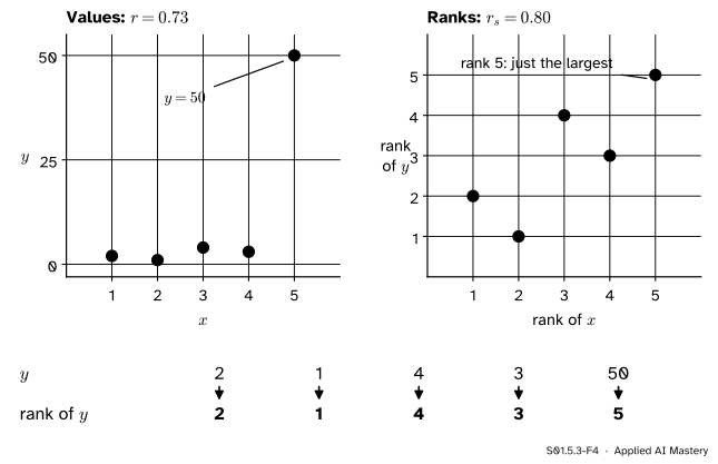
Spearman by hand, on five points with one outlier. Take the course’s five points and change the last \(y\) from \(5\) to \(50\): \(x = 1, 2, 3, 4, 5\) and \(y = 2, 1, 4, 3, 50\).
S01.5.3-F4
The value 50 becomes rank 5. Pearson’s \(r\) on the values is \(0.73\); on the ranks it is \(0.80\).
Pearson on the values. The means are \(\bar{x} = 3\) and \(\bar{y} = 12\). The \(y\)-deviations are \(-10, -11, -8, -9, 38\) and the \(x\)-deviations \(-2, -1, 0, 1, 2\), so the products are \(20, 11, 0, -9, 76\), which add to \(98\), and \(s_{xy} = {98 / 4} = 24.5\). The squared \(y\)-deviations add to \(1810\), so \(s_y = {\sqrt{1810 / 4}} = 21.27\), while \(s_x = 1.581\). Then
\[
r = \frac{24.5}{1.581 \times 21.27} = 0.73 .
\]
Spearman on the ranks. The \(x\) values are already ranks \(1, \dots, 5\). The \(y\) values \(2, 1, 4, 3, 50\) have ranks \(2, 1, 4, 3, 5\): 50 is simply the largest. The ranks are the course’s five points exactly, whose \(r\) is \(0.8\) (S01.5.2). So \(r_s = 0.80\), the same as before the outlier was planted. Make the last value 500 or 5 million and \(r_s\) stays \(0.80\), while \(r\) keeps falling towards \(0.71\), its value when one huge \(y\) outweighs all the rest. The code below checks 500.
Code
The quartet typed in from Anscombe’s table, and its summaries computed from scratch.
import mathx123 = [10, 8, 13, 9, 11, 14, 6, 4, 12, 7, 5]quartet = {"I": (x123, [8.04, 6.95, 7.58, 8.81, 8.33, 9.96, 7.24, 4.26, 10.84, 4.82, 5.68]),"II": (x123, [9.14, 8.14, 8.74, 8.77, 9.26, 8.10, 6.13, 3.10, 9.13, 7.26, 4.74]),"III": (x123, [7.46, 6.77, 12.74, 7.11, 7.81, 8.84, 6.08, 5.39, 8.15, 6.42, 5.73]),"IV": ([8, 8, 8, 8, 8, 8, 8, 19, 8, 8, 8], [6.58, 5.76, 7.71, 8.84, 8.47, 7.04, 5.25, 12.50, 5.56, 7.91, 6.89]),}def mean(v):returnsum(v) /len(v)def var(v): m = mean(v)returnsum((a - m) **2for a in v) / (len(v) -1)def pearson(x, y): mx, my = mean(x), mean(y) sxy =sum((a - mx) * (b - my) for a, b inzip(x, y)) / (len(x) -1)return sxy / math.sqrt(var(x) * var(y))def ranks(v):"""Rank from 1; tied values share the average of their ranks.""" order =sorted(v)return [mean([k +1for k, w inenumerate(order) if w == a]) for a in v]def spearman(x, y):return pearson(ranks(x), ranks(y))summary = {}for name, (x, y) in quartet.items(): r = pearson(x, y) w = r * math.sqrt(var(y) / var(x)) summary[name] = (mean(x), mean(y), var(x), var(y), r, mean(y) - w * mean(x), w, spearman(x, y))print(name, " ".join(f"{v:.3f}"for v in summary[name]))
I 9.000 7.501 11.000 4.127 0.816 3.000 0.500 0.818
II 9.000 7.501 11.000 4.128 0.816 3.001 0.500 0.691
III 9.000 7.500 11.000 4.123 0.816 3.002 0.500 0.991
IV 9.000 7.501 11.000 4.123 0.817 3.002 0.500 0.500
Each row prints the mean of \(x\) and of \(y\), both variances, \(r\), the intercept and slope of the trend line, and \(r_s\). Now the other numbers of this lesson, and the library calls: scipy.stats.spearmanr returns \(r_s\) (with a p-value, which is S02’s business), and pandas has DataFrame.corr(method="spearman").
import numpy as npimport pandas as pdfrom scipy import statsxs = [-2, -1, 0, 1, 2]print("y = x^2:", pearson(xs, [v * v for v in xs]), spearman(xs, [v * v for v in xs]))area = [55, 75, 25, 60, 155, 70, 35, 30, 35] # the flats table (invented)rent = [7, 12, 3, 10, 30, 8, 9, 4, 7]print("flats r:", round(pearson(area, rent), 2), " without F5:", round(pearson(area[:4] + area[5:], rent[:4] + rent[5:]), 2))print("flats r_s:", round(stats.spearmanr(area, rent).statistic, 2)," without F5:", round(stats.spearmanr(area[:4] + area[5:], rent[:4] + rent[5:]).statistic, 2))x5 = [1, 2, 3, 4, 5]for last in (50, 500): y = [2, 1, 4, 3, last]print(f"last y = {last}: r = {pearson(x5, y):.3f} r_s = {spearman(x5, y):.2f}")x3, y3 = quartet["III"]keep = [i for i inrange(11) if y3[i] !=12.74]slope, intercept = np.polyfit([x3[i] for i in keep], [y3[i] for i in keep], 1)print("set III without its outlier:", round(intercept, 2), round(slope, 3))print(pd.DataFrame({"x": quartet["IV"][0], "y": quartet["IV"][1]}).corr(method="spearman").round(2))
y = x^2: 0.0 0.0
flats r: 0.96  without F5: 0.78
flats r_s: 0.89  without F5: 0.84
last y = 50:  r = 0.728  r_s = 0.80
last y = 500:  r = 0.709  r_s = 0.80
set III without its outlier: 4.01 0.345
     x    y
x  1.0  0.5
y  0.5  1.0
The least-squares line through set III’s ten ordinary points is \(y = {4.01 + 0.345x}\), a whisker from the \({4 + 0.346x}\) that Anscombe printed. As the last value grows from 50 to 500, \(r\) drops from \(0.73\) to \(0.71\) and \(r_s\) does not move.
Explore
S01.5-X1
Anscombe explorer
Load any of Anscombe’s four sets, then drag a point, or choose it and move it with the sliders, or remove it. The table of summaries and the trend line follow. Press Hide the plot to see how little the table alone tells you.
Things to try. In set III, drag the outlier down onto the line of the other ten: \(r\) jumps to almost \(1\). In set IV, remove the far point: with every \(x\) equal to 8 there is no \(s_x\), and \(r\) cannot be computed. In set I, drag any one point to the bottom right corner, \(x = 20\) and \(y = 2\): \(r\) falls from \(0.82\) to near \(0\), while \(r_s\), which sees only one point out of order, stays between \(0.3\) and \(0.42\).
Pitfalls
S01.5.3-F5
Wrong beside right. From \(r = 0.82\) alone you picture a loose line. Set III is an almost perfect line and one outlier, and only the plot says so.
“\(r\) is close to 0, so the columns are unrelated.”
\(r\) sees only straight lines. \(y = x^2\) on \(x = -2, \dots, 2\) has \(r = 0\) and \(r_s = 0\) while \(x\) fixes \(y\) exactly. In machine learning a feature with \({r \approx 0}\) against the target can still be the most useful one for a model that can bend, such as a decision tree.
“\(r\) is high, so a straight line is the right description.”
Set II has \(r = 0.816\) and is a curve. A high \(r\) says a line does better than a flat line, not that a line is the right shape. Look at the plot, and at the misses from the line (ML01.4.4).
“The outlier spoils \(r\), so delete it.”
Deleting a value silently changes the data to suit the summary. Check it for a recording error, then report both: \(r = 0.96\) with the penthouse and \(0.78\) without, or the resistant \(r_s\) (S01.4.4 gives the rules for flagging and deciding).
Check yourself
Recall
1. What do Anscombe’s four sets have in common, and how do they differ?
Show answer
Each has \(n = 11\), means 9 and 7.50, variances 11 and about 4.12, \(r = 0.816\) and the trend line \(\hat{y} = {3 + 0.5x}\). One is a straight cloud, one a curve, one a line with an outlier and one a stack with one far point.
2. What is \(r\) for \(y = x^2\) on \(x = -2, \dots, 2\), and why?
Show answer
Exactly \(0\). The sum of products is the sum of \(x_i^3\) minus \(2\) times the sum of \(x_i\), and the cubes cancel in pairs. \(r\) measures only straight-line association.
3. How does the penthouse change the correlation of area and rent?
Show answer
With it \(r = 0.96\); without it \(r = 0.78\). One point makes most of the strength.
4. How is Spearman’s rank correlation computed, and how are ties handled?
Show answer
Rank each column, then compute Pearson’s \(r\) on the ranks. Tied values get the average of the ranks they share.
5. Why is Spearman’s \(r_s\)\(0.99\) for set III?
Show answer
Its ten ordinary points rise together almost perfectly in step; only the outlier is out of order, and a rank cannot be far out, so the rankings almost agree.
Exercises
1.★ Compute \(r_s\) by hand for \(x = 10, 20, 30, 40\) and \(y = 1, 3, 2, 100\).
Show solution
The ranks of \(x\) are \(1, 2, 3, 4\) and those of \(y\) are \(1, 3, 2, 4\). Both have mean \(2.5\). The deviations are \(-1.5, -0.5, 0.5, 1.5\) and \(-1.5, 0.5, -0.5, 1.5\), so the products are \(2.25, -0.25, -0.25, 2.25\), adding to \(4\). Each column’s squared deviations add to \(5\), so
2.★★ Compute \(r\) and \(r_s\) for \(x = 0, 1, 2, 3, 4\) and \(y = x^2\). What does the pair tell you?
Show solution
The means are \(\bar{x} = 2\) and \(\bar{y} = {(0 + 1 + 4 + 9 + 16)/5} = 6\). The deviations are \(-2, -1, 0, 1, 2\) and \(-6, -5, -2, 3, 10\), with products \(12, 5, 0, 3, 20\), adding to \(40\), so \(s_{xy} = 10\). Then \(s_x = {\sqrt{10/4}} = 1.581\), and the squared \(y\)-deviations add to \(174\), so \(s_y = {\sqrt{174/4}} = 6.595\). So
\[
r = \frac{10}{1.581 \times 6.595} = 0.96 .
\]
Here \(y\) rises whenever \(x\) does, so the ranks agree exactly and \(r_s = 1\). A curve can have a large \(r\), and a perfect monotone curve has \(r_s = 1\) but \(r < 1\).
3.★★★ Suppose the \(x\) values come in pairs \(a\) and \(-a\) (with \(0\) allowed once), and \(y_i = x_i^2\). Prove that \(r = 0\).
Show solution
The values pair off as \(a\) and \(-a\), so they add to \(0\) and \(\bar{x} = 0\); each \(x\)-deviation is \(x_i\). The sum of products is
In each pair, \({a^3 + (-a)^3} = 0\), and \(0^3 = 0\), so the sum of cubes is \(0\). The covariance is \(0\), so \(r = 0\) (assuming the \(x\) values are not all \(0\), so that \({s_x > 0}\), and so not all \(y\) equal).
Summary card
Plot before you summarise: one \(r\) fits very different pictures.
S01.5.3-F1
Same summaries, four pictures.
Straight lines only.\(y = x^2\) on \(-2, \dots, 2\) has \(r = 0\).
One point can make \(r\). Flats: \(0.96\) with the penthouse, \(0.78\) without.
Spearman.\(r_s\) is \(r\) on ranks; ties share the average rank; it measures monotone association.
Quartet.\(r = 0.82\) for all four; \(r_s = 0.82, 0.69, 0.99, 0.50\).
Sources and next steps
Sources. Each was opened and checked against this lesson on 12 November 2026.
F. J. Anscombe, Graphs in Statistical Analysis, The American Statistician 27(1), 1973, pages 17 to 21. Page 19 holds the table of the four sets, their shared output (\(n = 11\), means 9.0 and 7.5, regression line \(y = {3 + 0.5x}\)) and the remark that all but one point of set 3 lie close to the line \(y = {4 + 0.346x}\).
NIST/SEMATECH, e-Handbook of Statistical Methods, Section 1.1.6. Works the four sets with their shared statistics, including correlation 0.816 (0.817 for set 4), and concludes that the data should be plotted.
Allen B. Downey, Think Stats, third edition, Chapter 7. Section 7.4: for a non-linear relationship the correlation can be close to 0. Section 7.5: rank correlation, also called Spearman’s, computed on the ranks of the values.
Rafael A. Irizarry, Introduction to Data Science, Chapter 19. Section 19.2 shows one outlier driving a correlation of 0.988 and the rank correlation falling close to 0.
SciPy developers, scipy.stats.spearmanr and scipy.stats.rankdata, SciPy 1.18. The first returns the statistic and a p-value; the second ranks with the default method ‘average’, which gives tied values the average of their ranks.