The empirical distribution function draws a column as a staircase that climbs by 1/n at every value. Build it by hand for nine rents, read the median, the quartiles and any share straight off it, and compare two groups with no bins to choose.
Build the empirical distribution function of a small data set by hand, including the larger jump at a repeated value.
Read the median, the quartiles, any percentile and the share of values in an interval off a staircase.
Explain why a staircase needs no bins and why its quantile reading can differ from NumPy’s default rule.
Compare two groups by laying their staircases on one plot, and compute the staircase with a sort, with scipy.stats.ecdf and with numpy.quantile.
In review. The maths and code on this page are checked by automated tests on every change, but an independent reader has not signed it off yet. Spot a mistake or a confusing step? Tell us.
The question
What share of the nine flats rent for 1,000 euros a month or less? Below what rent do half of them fall? A histogram can only hint, because its answer depends on where the bins were cut. Is there a picture that answers both questions exactly, shows every value, and asks you to choose nothing?
From the last lesson
1. With bins of width 5 starting at 0, which bin holds the rent 10?
Show answer
The bin from 10 to 15: each bin keeps its left edge and drops its right edge.
2. What does the area of a bar mean on the density scale?
Show answer
The share of the data in that bin. Density is the proportion divided by the width, so height times width gives the proportion back, and the areas add to 1.
Intuition
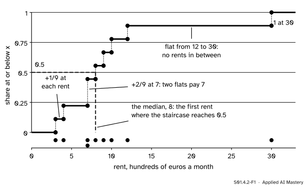
Stand at any rent \(x\) on the number line and ask: what share of the nine rents are at or below\(x\)? Below 3 the answer is 0. At 3 it becomes 1/9. It stays 1/9 until 4, where it becomes 2/9. At 7 it jumps by 2/9 at once, because two flats pay 7. After the last rent, 30, the answer is 1 for good.
Draw that answer for every \(x\) and you get a staircase: flat between rents, with a step up at each one. It is called the empirical cumulative distribution function, or ECDF.
S01.4.2-F1
The ECDF of the nine rents. Each rent lifts the staircase by 1/9; the two flats at 7 lift it by 2/9. The staircase crosses 0.5 at the median, 8.
The staircase hides nothing. Each step sits exactly at a value, so every rent can be read back off it. Where values crowd together the staircase climbs steeply; where they are sparse it runs flat, like the long flat stretch from 12 to 30. And no one had to choose a bin.
Build it up
Step 1. Sort. Write the rents in order: 3, 4, 7, 7, 8, 9, 10, 12, 30. In the course notation they are \(x_{(1)} \le x_{(2)} \le \dots \le x_{(9)}\).
Step 2. Count at or below. For any \(x\), count the rents that are at most \(x\). For \(x = 10\) the rents 3, 4, 7, 7, 8, 9 and 10 qualify: seven of them.
Step 3. Divide by \(n\). The share at or below 10 is \(7/9 = 0.78\). Seventy-eight percent of the flats rent for 1,000 euros a month or less. That answers the first question of the hook.
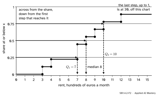
Step 4. Read across, then down. To find the rent below which a given share \(q\) falls, start at \(q\) on the vertical axis, go across to the first step that reaches the line, and go down.
S01.4.2-F2
Quantiles read off the staircase: across from 0.25, 0.5 and 0.75, down to \(Q_1 = 7\), the median 8 and \(Q_3 = 10\).
At 0.25 the staircase is still at 2/9 = 0.22 after the rent 4, and first reaches 0.25 at 7, where it jumps to 4/9. So the first quartile is 7. At 0.5 it reaches 5/9 at 8, and at 0.75 it reaches 7/9 at 10. These are the quartiles of S01.3.2: 7, 8 and 10.
Step 5. What the staircase has that the histogram lacks. No bins to choose, so no two analysts can draw it differently. Every value is visible as a step. And any share, of any interval, is read off it exactly, as the next section shows.
The formal statement
NoteDefinition: empirical distribution function
For values \(x_1, \dots, x_n\), the empirical cumulative distribution function at a number \(x\) is the share of the values that are at most \(x\):
For a share \(q\) between 0 and 1, the value read off the staircase is the smallest data value \(x\) with \(\hat F(x) \ge q\).
Four properties follow, each from counting.
1. It never goes down. If \(x < y\), every value at most \(x\) is also at most \(y\), so the count at \(y\) is at least the count at \(x\).
2. It runs from 0 to 1. Below \(x_{(1)}\) no value qualifies, so \(\hat F = 0\). At \(x_{(n)}\) and beyond every value qualifies, so \(\hat F = 1\).
3. The jump at a value is its share. Just below a value \(v\), the count is the number of values less than \(v\). At \(v\) it is the number at most \(v\). The difference is the number of values equal to \(v\). So the staircase jumps by \(1/n\) at a value that occurs once and by \(2/n\) at a value that occurs twice, as at the rent 7.
4. The share in an interval is a difference. For \(a < b\), the values at most \(b\) are those at most \(a\) together with those above \(a\) and at most \(b\). Counting both sides and dividing by \(n\), \({\hat F(b) = \hat F(a)}\) + (share in \((a, b]\)), so
For the rents, the share above 5 and at most 10 is \({\hat F(10) - \hat F(5) = 7/9 - 2/9 = 5/9}\): the rents 7, 7, 8, 9 and 10.
Reading versus interpolating. The read-off rule picks a data value. NumPy calls it method="inverted_cdf". The course’s quantile rule (S01.3.2, NumPy’s default "linear") instead places the \(q\)-quantile at position \({(n - 1)q}\) in the sorted values and draws a straight line between neighbours. For the nine rents the two agree at the quartiles. They part company at the 90th percentile: the staircase first reaches 0.9 at 30, while the default rule interpolates between \(x_{(8)} = 12\) and \(x_{(9)} = 30\) at position \({8 \times 0.9 = 7.2}\) counted from 0:
\[
12 + 0.2 \times (30 - 12) = 15.6 .
\]
Both are legitimate quantile rules; a report says which one it used.
Worked example
Build the staircase of the nine rents by hand and read four things off it.
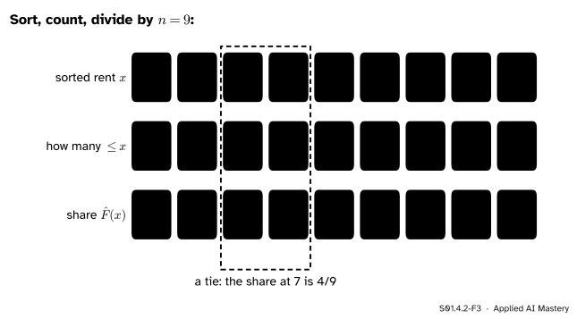
The table. Sort the rents and keep a running count. The share at each distinct rent is the count after its last copy, divided by 9.
S01.4.2-F3
Sort, count, divide by \(n = 9\). At a tie only the last copy sets the share: the staircase goes straight from 2/9 to 4/9 at the rent 7.
So the staircase has heights 1/9 at 3, 2/9 at 4, 4/9 at 7, 5/9 at 8, 6/9 at 9, 7/9 at 10, 8/9 at 12 and 1 at 30.
Four readings.
A share. At most 10: \({\hat F(10) = 7/9 = 0.78}\).
A tail. Above 12: \({1 - \hat F(12) = 1 - 8/9 = 1/9}\), the penthouse alone.
An interval. Above 4 and at most 9: \({\hat F(9) - \hat F(4) = 6/9 - 2/9 = 4/9}\), the rents 7, 7, 8 and 9.
A quantile. The median: \(\hat F(7) = 4/9 = 0.44\) is short of 0.5 and \({\hat F(8) = 5/9 = 0.56}\) is not, so the median is 8.
Code
From scratch, a sort and a running count give the steps, and a count gives \(\hat F\) at any \(x\).
rents = [3, 4, 7, 7, 8, 9, 10, 12, 30]def ecdf_steps(values):"""Distinct sorted values and the share of values at or below each.""" xs =sorted(values) n =len(xs) steps = {}for count, x inenumerate(xs, start=1): steps[x] = count / n # a later copy of x overwrites the earlier onereturnlist(steps), list(steps.values())def F(values, x):returnsum(v <= x for v in values) /len(values)def read_off(values, q):"""The smallest value whose share at or below reaches q.""" xs, shares = ecdf_steps(values)returnnext(x for x, s inzip(xs, shares) if s >= q -1e-12)xs, shares = ecdf_steps(rents)print("steps:", [(x, f"{round(s *9)}/9") for x, s inzip(xs, shares)])print("F(10) =", round(F(rents, 10), 3), " above 12:", round(1- F(rents, 12), 3)," (4, 9]:", round(F(rents, 9) - F(rents, 4), 3))print("read off: Q1, median, Q3, 90th =", [read_off(rents, q) for q in (0.25, 0.5, 0.75, 0.9)])
The library versions. scipy.stats.ecdf returns an object whose cdf holds the step positions (quantiles) and heights (probabilities) and can evaluate the staircase anywhere. numpy.quantile reads quantiles with either rule.
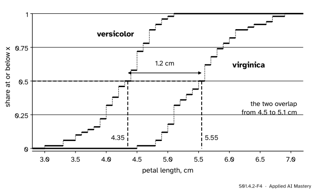
Two groups. The petal lengths of the 50 versicolor and the 50 virginica flowers in scikit-learn’s iris data, each as its own staircase.
from sklearn.datasets import load_irisiris = load_iris()petal, species = iris.data[:, 2], iris.targetversi, virgi = petal[species ==1], petal[species ==2]for name, v in [("versicolor", versi), ("virginica", virgi)]: e = stats.ecdf(v)print(f"{name:10s} median {np.median(v):.2f} share at or below 4.5 cm: {e.cdf.evaluate(4.5):.2f}"f" range {v.min()} to {v.max()}")
versicolor median 4.35  share at or below 4.5 cm: 0.72  range 3.0 to 5.1
virginica  median 5.55  share at or below 4.5 cm: 0.02  range 4.5 to 6.9
Matplotlib draws a staircase with Axes.ecdf(values), one call per group on the same axes.
Explore
The module’s interactive, the histogram bin-width explorer, lives in S01.4.1. Open it beside this picture: the two clumps it shows at narrow widths are the steep stretches of a staircase, and they need no width here.
S01.4.2-F4
Two species, two staircases. Virginica’s lies to the right at every share, so at every percentile its petals are longer; the medians differ by 1.2 cm.
Read it the way you read one staircase. Across from 0.5, the medians are 4.35 and 5.55 cm. Up from 4.5 cm, 72 percent of versicolor petals are at most that long, but only 2 percent of virginica petals. Where one staircase lies wholly to the right of the other, one group has larger values at every share, a stronger statement than “its mean is bigger”. The same plot is how a feature’s values in new data are compared with its values in the training data (E05.4).
Pitfalls
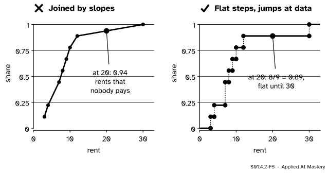
S01.4.2-F5
Wrong beside right. Sloping lines between the points invent rents between 12 and 30. The staircase stays flat where there are no data.
“Join the points with lines; it looks smoother.”
A line from (12, 8/9) to (30, 1) says that some flats rent for 20, and reads 0.94 there. No flat does: the true share at or below 20 is 8/9 = 0.89. The ECDF changes only at data values, so it is flat between them.
“At a jump, the value is the bottom of the step.”
\(\hat F(7)\) counts the rents at or below 7, so it includes both 7s: 4/9, the top of the step. The bottom, 2/9, is the share strictly below 7. In the figures a filled dot marks the value and a hollow dot the point it is not.
“A percentile is a percentile.”
The 90th percentile of the nine rents is 30 read off the staircase and 15.6 by NumPy’s default. Small samples make the rules disagree most. State the rule, or report the share instead, which is never ambiguous.
“Where the staircase is high, the values are common.”
Height is the running total, so it is always highest at the right. Common values show as steepness: the staircase climbs fast where values crowd together, which is where a histogram has its tall bars.
Check yourself
Recall
1. What does \(\hat F(x)\) measure?
Show answer
The share of the values that are at most \(x\).
2. How big is the jump of the staircase at a value that occurs \(k\) times among \(n\) values?
Show answer
\(k/n\): the count at the value minus the count just below it is the number of copies.
3. How do you read the median off a staircase?
Show answer
Go across from 0.5 to the first step that reaches 0.5 and read the value below it. For the nine rents that is 8.
4. How do you get the share of values above \(a\) and at most \(b\) from the staircase?
Show answer
\({\hat F(b) - \hat F(a)}\).
5. Name two advantages of the ECDF over a histogram.
Show answer
There are no bins to choose, so it cannot be drawn two ways, and every value is visible as a step. Shares and quantiles can be read off it exactly.
Exercises
1.★ From the staircase of the nine rents, find \(\hat F(9)\), the share of rents above 9 and the share above 4 and at most 9.
Show solution
Six rents are at most 9 (3, 4, 7, 7, 8, 9), so \({\hat F(9) = 6/9 = 2/3}\). The share above 9 is \({1 - 2/3 = 1/3}\): the rents 10, 12 and 30. The share in \((4, 9]\) is \({\hat F(9) - \hat F(4) = 6/9 - 2/9 = 4/9}\): the rents 7, 7, 8 and 9.
2.★★ A tenth flat with rent 8 joins the table. Give the new heights of the staircase at each distinct rent, the size of the jump at 8, and the median read off the staircase. Does it agree with the course’s quantile rule?
Show solution
Sorted: 3, 4, 7, 7, 8, 8, 9, 10, 12, 30, so \(n = 10\). The running counts after the last copy of each rent are 1, 2, 4, 6, 7, 8, 9, 10, giving heights 0.1, 0.2, 0.4, 0.6, 0.7, 0.8, 0.9 and 1 at 3, 4, 7, 8, 9, 10, 12 and 30. The jump at 8 is \({0.6 - 0.4 = 0.2 = 2/10}\), for its two copies. The first height to reach 0.5 is 0.6 at 8, so the median read off is 8. The course’s rule puts the median at position \({9 \times 0.5 = 4.5}\), halfway between \(x_{(5)} = 8\) and \(x_{(6)} = 8\), which is also 8. They agree.
3.★★★ Take \(n\) distinct values. Show that for odd \({n = 2m + 1}\) the median read off the staircase is the middle value \(x_{(m+1)}\), and find what it gives for even \({n = 2m}\).
Show solution
With distinct values, exactly \(k\) values are at most \(x_{(k)}\), so \({\hat F(x_{(k)}) = k/n}\). The read-off median is the first \(x_{(k)}\) with \({k/n \ge 1/2}\), that is with \({k \ge n/2}\).
For \({n = 2m + 1}\) this asks for \({k \ge m + 1/2}\). The smallest whole number that qualifies is \({k = m + 1}\), so the median is \(x_{(m+1)}\), the middle value.
For \({n = 2m}\) it asks for \({k \ge m}\), so the staircase gives \(x_{(m)}\), the lower of the two middle values. The staircase is at exactly 0.5 all the way from \(x_{(m)}\) to \(x_{(m+1)}\), so every point of that step splits the data in half; the usual median takes the midpoint of the step. The same can happen with ties: exactly 25 of the 50 versicolor petals are at most 4.3 cm, so their staircase is at 0.5 from 4.3 up to 4.4 cm, and the median is 4.35 cm.
Summary card
The ECDF is the share at or below \(x\): a staircase with no bins.
S01.4.2-F1
Climb 1/n at every value.
Definition.\(\hat F(x)\) = (number of \(x_i \le x\)) / \(n\).
Jumps.\(k/n\) at a value with \(k\) copies; flat between values.
Shares. Share in \((a, b]\) is \({\hat F(b) - \hat F(a)}\).
Quantiles. Across from \(q\), down from the first step that reaches it.
Sources and next steps
Sources. Each was opened and checked against this lesson on 12 November 2026.
SciPy, scipy.stats.ecdf. The ECDF as a step-function estimate of the CDF, and its cdf.quantiles, cdf.probabilities and evaluate.
NumPy, numpy.quantile. The default method ‘linear’ and the method ‘inverted_cdf’, which follows from the empirical distribution function, numbered after Hyndman and Fan (1996).
Next.S01.4.3 Anatomy of a boxplot draws three of these quantiles as a box and uses them to flag values that sit far out.