Two columns can share their mean and standard deviation and still look nothing alike. Standardise values into z-scores, measure lopsidedness with the skewness, read modes and tails from dot plots, and choose the summaries that fit the shape.
Standardise a column into z-scores and prove that they have mean 0 and standard deviation 1.
Compare values measured in different units by their z-scores.
Compute the skewness g1 by hand and read its sign as the side of the long tail.
Tell one mode from two, and light tails from heavy ones, on a dot plot.
Choose between the median with the IQR and the mean with the standard deviation according to the shape of the data.
In review. The maths and code on this page are checked by automated tests on every change, but an independent reader has not signed it off yet. Spot a mistake or a confusing step? Tell us.
The question
Two columns of nine numbers both have mean 10 and standard deviation 8. One is the rents of the flats table; the other is invented. Reported as “10 plus or minus 8”, they are the same. Drawn as dots, they look nothing alike. What do the mean and the standard deviation leave out, and how do you measure it?
From the last lesson
1. What are the variance and the standard deviation of the nine rents?
Show answer
The squared deviations add to 512, so \({s^2 = 512 / 8 = 64}\) and \({s = 8}\) hundred euros.
2. Every value is changed to \({a x + b}\). What happens to the standard deviation?
Show answer
It is multiplied by \(\abs{a}\); the shift \(b\) has no effect.
Intuition
The shape of a column is what its dot plot looks like once you forget where it sits and how wide it is: whether it is lopsided, how many humps it has, and how far its thinnest parts reach.
S01.3.4-F1
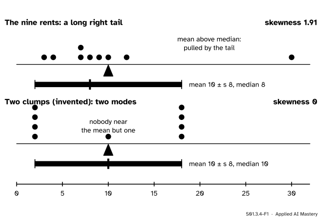
The same mean, the same standard deviation, the same band of mean plus or minus \(s\). The rents have a long right tail and the mean sits above the median; the invented set has two clumps and almost nobody near the mean.
Three words describe shape. A column is skewed when one tail is longer than the other: the rents trail off to the right, so they are skewed right, and the long tail drags the mean above the median. A mode is a peak: the rents have one (the most common rent is 7), the invented set has two clumps, and a summary that names one “typical value” misleads for it. Tails are the thin ends; heavy tails mean more values far from the centre than an evenly spread set would have.
Before measuring any of this, there is a tool that makes shape easier to see: measure every value from the mean, in units of the standard deviation.
Build it up
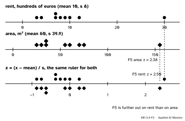
Step 1. A common ruler. The penthouse pays 30 when the mean rent is 10, and has 155 square metres when the mean area is 60. Which is further out? The raw distances, 20 hundred euros and 95 square metres, cannot be compared. Divide each by its column’s standard deviation (8 and 39.9) and both become counts of standard deviations: \({20 / 8 = 2.5}\) and \({95 / 39.9 = 2.38}\).
S01.3.4-F2
Standardising re-labels each ruler so that the mean sits at 0 and one standard deviation is one unit. The dots keep their pattern; only the numbers on the ruler change.
That count is the z-score. The rulers in the figure are stretched copies of each other, which is the point: a z-score changes the units, never the pattern.
Step 2. Cube the deviations. Squares lose the sign of a deviation, and the sign is exactly what tells left from right. Cubes keep it: \({(-2)^3 = -8}\) but \({2^3 = 8}\). Add the cubes, and a long right tail wins, because its far values, cubed, dwarf everything else. Scaled to have no units, that sum becomes the skewness.
Step 3. Count the humps. No single number in this lesson sees the second clump in the anchor figure. Its skewness is 0, like any set that is symmetric about its mean. You find modes by looking: a dot plot, or the histogram of S01.4.1.
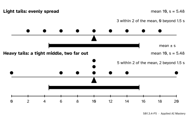
Step 4. Compare the tails. Two more invented sets of nine test marks, out of 20, share their mean and standard deviation but spread differently.
S01.3.4-F5
Light tails against heavy tails, with the same mean and the same \(s\). The heavy-tailed set packs more values near the middle and puts two further out: both effects at once keep \(s\) the same.
The formal statement
NoteDefinitions: z-score and skewness
The z-score of value \(x_i\) is \({z_i = (x_i - \bar{x}) / s}\): its distance from the mean in standard deviations. Replacing every value by its z-score is called standardising.
With \(m_k = {\frac{1}{n}\sum_{i=1}^{n} (x_i - \bar{x})^k}\) for the mean \(k\)-th power of the deviations (divisor \(n\)), the skewness is
\[
g_1 = \frac{m_3}{m_2^{3/2}} .
\]
Result 1: z-scores have mean 0 and standard deviation 1. Standardising is a change of the form \({z = a x + b}\) with \({a = 1/s}\) and \({b = -\bar{x}/s}\), since \({(x - \bar{x})/s} = {x/s - \bar{x}/s}\). By exercise 3 of S01.3.1 the new mean is
and by Result 1 of S01.3.3 the new standard deviation is \({\abs{1/s} \times s = 1}\). For the rents the z-scores are −0.875, −0.75, −0.375, −0.375, −0.25, −0.125, 0, 0.25, 2.5; they add to 0 and their squares add to 8, so their variance is \({8/8 = 1}\).
This is the feature scaling that P02.2.4 computed and that lesson ML01.3.3 needs: a distance between flats that adds square metres to hundreds of euros is dominated by whichever column has the bigger numbers, until both are standardised.
Result 2: what \(g_1\) measures. Three facts follow from the definition.
Sign. Positive cubes come from values above the mean, negative cubes from values below. A long right tail has a few large positive cubes that outweigh the rest, so \({g_1 > 0}\); a long left tail gives \({g_1 < 0}\).
No units. Under \({y = a x + b}\) every deviation is multiplied by \(a\) (S01.3.3), so \(m_3\) is multiplied by \(a^3\) and \({m_2^{3/2}}\) by \(\abs{a}^3\). For \({a > 0}\) these cancel: rents in euros have the same skewness as rents in hundreds of euros, and so do their z-scores.
Symmetry gives zero. If the values are symmetric about their mean, each deviation \(d\) has a partner \({-d}\), the cubes cancel in pairs and \({g_1 = 0}\). The two clumps and both test-mark sets have \({g_1 = 0}\).
Two conventions. SciPy’s scipy.stats.skew returns \(g_1\) by default. pandas returns an adjusted value, \({G_1} = {g_1 \sqrt{n(n-1)}/(n-2)}\), meant to correct a bias in small samples. For \({n = 9}\) the factor is \({{\sqrt{72}/7} \approx 1.21}\), so pandas reports 2.32 where SciPy reports 1.91. For large \(n\) the factor tends to 1 and the two agree.
The rule that follows. The mean and the standard deviation are built from deviations and squared deviations, so a long tail or a far value pulls both (S01.3.1, S01.3.3). The median and the IQR count positions, so a far value barely moves them (S01.3.2).
For data that are roughly symmetric with one mode, report the mean and the standard deviation.
For skewed data, or data with far values, report the median and the IQR, and say what is in the tail.
For data with two or more modes, report neither alone: describe the groups, and look for the column that separates them.
Go deeper: the fourth power, and why tails need more than one number
The same recipe with fourth powers gives the kurtosis, \({m_4 / m_2^2}\), often reported minus 3 as the “excess kurtosis”. A fourth power weights far values even more than a cube and ignores their side, so a high kurtosis signals heavy tails or outliers. For the two test-mark sets it is \({-1.23}\) (light) against \({0.21}\) (heavy), excess, in SciPy’s default. With nine values such a number is very unstable; a dot plot shows the same thing more reliably. The tails get their own tools in S01.4.4.
Worked example
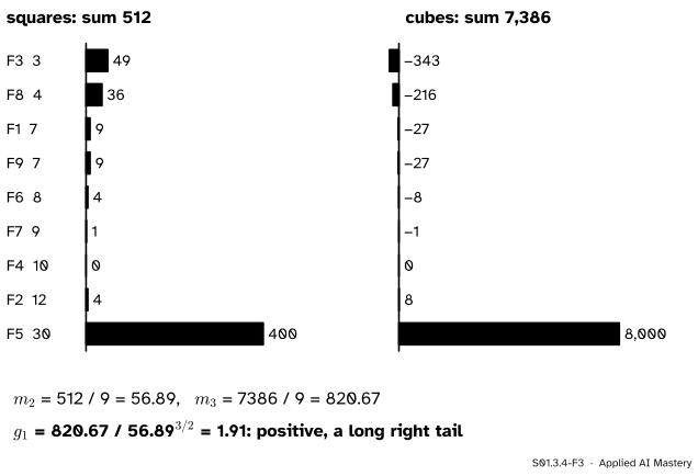
The skewness of the nine rents, by hand. The deviations from 10 are −7, −6, −3, −3, −2, −1, 0, 2, 20.
S01.3.4-F3
Squaring makes the penthouse large; cubing makes it overwhelming, and keeps its sign. The six negative cubes add to only \({-622}\) against the penthouse’s \({+8000}\).
Squares.\(49 + 36 + 9 + 9 + 4 + 1 + 0 + 4 + 400 = 512\), so \({m_2 = 512/9 \approx 56.89}\). (Divisor \(n\), not \({n - 1}\): that is part of the definition of \(g_1\).)
Cubes. The negatives add to \(-343 - 216 - 27 - 27 - 8 - 1 = -622\); the positives to \({8 + 8000 = 8008}\). In total \(7386\), so \({m_3 = 7386/9 \approx 820.67}\).
Positive and large: a long right tail, as the dot plot showed. The mean (10) sits above the median (8), on the side of the tail. Without the penthouse the skewness is \({-0.14}\), close to symmetric (exercise 2).
Code
From scratch first: z-scores and the skewness.
import mathrents = [7, 12, 3, 10, 30, 8, 9, 4, 7] # F1 to F9, hundreds of euros a monthareas = [55, 75, 25, 60, 155, 70, 35, 30, 35] # square metresdef mean(v):returnsum(v) /len(v)def sd(v): m = mean(v)return math.sqrt(sum((x - m) **2for x in v) / (len(v) -1))def z_scores(v): m, s = mean(v), sd(v)return [(x - m) / s for x in v]def skewness(v): m = mean(v) m2 =sum((x - m) **2for x in v) /len(v) m3 =sum((x - m) **3for x in v) /len(v)return m3 / m2 **1.5z = z_scores(rents)print("z of the rents:", [round(x, 3) for x in z])print("mean", round(mean(z), 12), " sd", round(sd(z), 12))print("penthouse: rent z", z[4], " area z", round(z_scores(areas)[4], 2))print("skewness:", round(skewness(rents), 2), " of the z-scores:", round(skewness(z), 2))
z of the rents: [-0.375, 0.25, -0.875, 0.0, 2.5, -0.25, -0.125, -0.75, -0.375]
mean 0.0  sd 1.0
penthouse: rent z 2.5   area z 2.38
skewness: 1.91   of the z-scores: 1.91
Now the shapes of the four invented sets, and the two library conventions for skewness.
two clumps: mean 10, s 8.00, median 10, skew 0.00
     light: mean 10, s 5.48, median 10, skew 0.00
     heavy: mean 10, s 5.48, median 10, skew 0.00
scipy: 1.91   pandas: 2.32   factor: 1.212
stats.skew(rents, bias=False) gives the same 2.32 as pandas. Whichever you report, say which.
Explore
This module’s interactive, Balance and middle, lives in lesson S01.3.3. Drag the penthouse towards the others until the rents look symmetric, and notice the mean and the median meet as the tail disappears.
Pitfalls
S01.3.4-F4
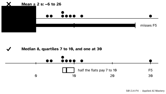
Wrong beside right. For skewed rents, mean plus or minus two standard deviations runs below zero and still misses the one unusual flat. The median and quartiles describe the bulk, and the penthouse is named on its own.
“Mean plus or minus two standard deviations holds nearly all the data.”
That rule of thumb belongs to symmetric, single-humped data, and the normal curve of M06 makes it precise. For the skewed rents the band runs from \({-6}\), an impossible rent, to 26, and the only flat that stands out lies outside it. Check the shape before you use the band.
“Standardising makes the data normal, or removes the outliers.”
Standardising is a change of unit. It moves and stretches the ruler and leaves the pattern alone: the z-scores of the rents have skewness 1.91, the same as the rents, and the penthouse is still far out, at \({z = 2.5}\). To reduce a long right tail you need a transformation that bends the ruler, such as \(\log_{10}\), which S01.4.4 uses.
“SciPy says 1.91 and pandas says 2.32, so one of them is wrong.”
They compute different, documented quantities: \(g_1\) and the adjusted \(G_1\). In small samples the difference is large, at \({n = 9}\) about a fifth. State the convention, and use one convention for every column you compare.
Check yourself
Recall
1. What is the z-score of the penthouse’s rent of 30, given mean 10 and \({s = 8}\)?
Show answer
\({(30 - 10) / 8 = 2.5}\): two and a half standard deviations above the mean.
2. Why do z-scores always have mean 0 and standard deviation 1?
Show answer
Standardising is \({z = x/s - \bar{x}/s}\), a change of unit and a shift. The mean becomes \({\bar{x}/s - \bar{x}/s = 0}\) and the standard deviation becomes \({s/s = 1}\).
3. What is the sign of the skewness for a long right tail, and why?
Show answer
Positive. The far values on the right have large positive cubed deviations that outweigh the small negative cubes of the values on the left.
4. Name two columns with the same mean and standard deviation but different shapes.
Show answer
The rents (3, 4, 7, 7, 8, 9, 10, 12, 30: one mode, a long right tail) and the invented two clumps (2, 2, 2, 2, 10, 18, 18, 18, 18: two modes, symmetric). Both have mean 10 and \({s = 8}\).
5. Which summaries should you report for a skewed column, and which for a roughly symmetric one?
Show answer
The median and the IQR for skewed data; the mean and the standard deviation for roughly symmetric, single-humped data.
Exercises
1.★ Flat F2 pays 12 and has 75 square metres. Find the z-score of each, given rent mean 10 with \({s = 8}\) and area mean 60 with \({s \approx 39.9}\). In which column is F2 further from the mean?
Show solution
Rent: \({(12 - 10)/8 = 0.25}\). Area: \({(75 - 60)/39.9 \approx 0.38}\). F2 is a little further out on area, measured in standard deviations, though both are well inside the bulk of their columns.
2.★★ Compute the skewness \(g_1\) of the eight rents left without the penthouse, 3, 4, 7, 7, 8, 9, 10, 12, whose mean is 7.5.
Show solution
The deviations are −4.5, −3.5, −0.5, −0.5, 0.5, 1.5, 2.5, 4.5. Their squares add to 62, so \({m_2 = 62/8 = 7.75}\). Their cubes are −91.125, −42.875, −0.125, −0.125, 0.125, 3.375, 15.625, 91.125, which add to \({-24}\), so \({m_3 = -24/8 = -3}\). Then \({m_2^{3/2}} = {7.75 \times \sqrt{7.75}} \approx {7.75 \times 2.784} \approx 21.58\), and \({g_1 = -3 / 21.58 \approx -0.14}\). Removing one flat turned a strong right skew into a column that is close to symmetric, with a slight lean to the left.
3.★★★ Prove that changing every value to \({y = a x + b}\) with \({a > 0}\) leaves \(g_1\) unchanged, and that \({a < 0}\) flips its sign.
Show solution
By S01.3.3, each deviation becomes \({y_i - \bar{y}} = {a\,(x_i - \bar{x})}\). Raise it to the power \(k\) and average: \({m_k(y) = a^k\,m_k(x)}\). So \({m_3(y) = a^3 m_3(x)}\), and since \({m_2(x) \ge 0}\),
Dividing, \({g_1(y) = (a^3 / \abs{a}^3)\, g_1(x)}\). The factor \({a^3/\abs{a}^3}\) is \({+1}\) when \({a > 0}\) and \({-1}\) when \({a < 0}\). A change of unit keeps the skewness; mirroring the values, as in \({y = -x}\), swaps the long tail to the other side and flips its sign.
Summary card
The mean and \(s\) give a place and a width; the shape is what they leave out.
S01.3.4-F1
Same mean, same \(s\), different shapes.
z-score.\({z_i = (x_i - \bar{x})/s}\): mean 0, standard deviation 1, shape unchanged.
Skewness.\({g_1 = m_3 / m_2^{3/2}}\): positive for a long right tail; 1.91 for the rents.
Choose. Skewed: median and IQR. Symmetric, one mode: mean and \(s\). Two modes: look for groups.
Sources and next steps
Sources. Each was opened and checked against this lesson on 12 November 2026.
NIST/SEMATECH, e-Handbook of Statistical Methods, Section 1.3.5.11, Measures of skewness and kurtosis: the Fisher-Pearson coefficient of skewness (third central moment over the cube of the standard deviation, both with divisor \(N\)), the adjusted coefficient with the factor \({\sqrt{N(N-1)}/(N-2)}\) that many programs report, positive values for data skewed right, and high kurtosis as a sign of heavy tails or outliers.
David Diez, Mine Cetinkaya-Rundel and Christopher Barr, OpenIntro Statistics, 4th edition (free PDF). Section 2.1.3 identifies skew by the long tail and names unimodal, bimodal and multimodal shapes; Figure 2.9 in Section 2.1.4 shows three very different distributions with the same mean and standard deviation.
SciPy documentation, scipy.stats.skew: the default bias=True returns \({g_1 = m_3/m_2^{3/2}}\) with \(m_i\) the biased central moments; bias=False returns the adjusted Fisher-Pearson coefficient \(G_1\).
pandas documentation, Series.skew: returns the unbiased skew, “normalized by N-1”; the code above confirms that it equals SciPy’s bias=False value, 2.32 for the rents.
Next. Module S01.4 draws whole distributions: histograms, the cumulative view, the boxplot of the five-number summary, and what to do with values flagged as outliers.