How samples go wrong: selection, non-response and survivorship
Convenience and volunteer samples, frames that leave units out, non-response and survivorship, each worked in counts and means. Derive why asking members instead of groups weights each group by its size, and ask of any data set who is missing and why.
Name the rule by which rows got into a table (convenience, volunteering, the frame, non-response, survival) and say which way it bends a mean.
Derive that asking members about their group gives the sum of the squared group sizes over the sum of the sizes, and compute it.
Explain why answers whose chance of arriving falls with the value average below the population mean at every sample size.
Put the two questions who is missing and why to a data set, and check what the table itself can reveal about them.
In review. The maths and code on this page are checked by automated tests on every change, but an independent reader has not signed it off yet. Spot a mistake or a confusing step? Tell us.
The question
A website asks tenants to report their rent. Over many weeks the reported rents average 7.1 (hundreds of euros a month), and the website announces that the typical flat in the city costs 710 euros. The true mean is 830. Every reported rent was true. So what went wrong, and how could you have suspected it from the data alone?
From the last lesson
1. Write the population mean in terms of the stratum means and their shares.
Show answer
\(\mu = \sum_g W_g\, \mu_g\) with \(W_g = N_g / N\); for the city \({0.5 \cdot 5} + {0.3 \cdot 8} + {0.2 \cdot 17} = 8.3\).
2. Why does the plain mean of the nine flats (10) miss the city’s mean (8.3)?
Show answer
The table holds three flats per district, so each district gets weight one third. Centre, the dearest, is a fifth of the city but a third of the table.
Intuition
Every row of a table came through a series of doors. The unit had to exist in the population, be on the list, be chosen, answer, and still be there when the counting was done. Each door has a rule, and a rule that lets some kinds of unit through more easily than others bends every summary of the table. Statisticians call such a rule selection, and the bent answer selection bias.
S01.2.4-F1
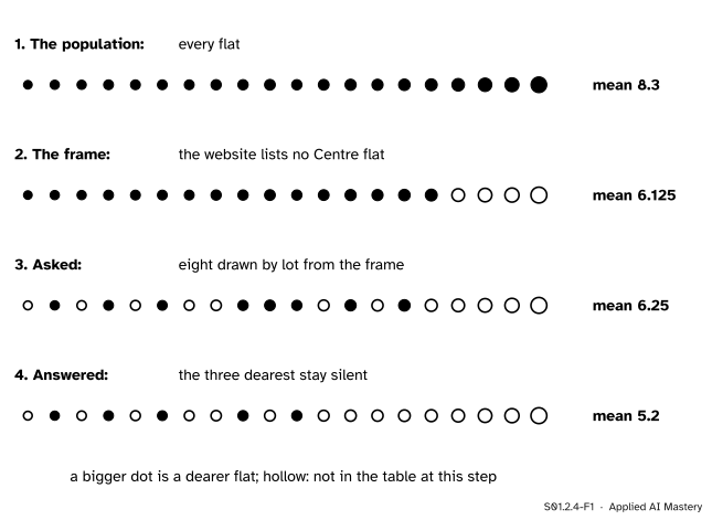
Twenty invented flats with the city’s mix of districts, passing through the doors into a table. The frame drops Centre; the draw by lot is fair; then the dearest of those asked stay silent. The mean falls from 8.3 to 5.2, and no row of the final table is wrong.
Look at which doors did the damage. The draw by lot moved the mean a little, by chance, from 6.125 to 6.25: that is the sampling variability of lesson S01.2.2. The other two doors moved it a long way and always in the same direction, because their rules depend on the rent. That is bias, and no larger sample would undo it.
Build it up
Here are the common doors, each with one small invented case in counts and means.
A convenience sample takes the units that are easy to reach. An agent who asks only the three flats in her own building in Centre (rents 12, 30 and 9) reports a mean of \(51 / 3 = 17\), twice the city’s 8.3.
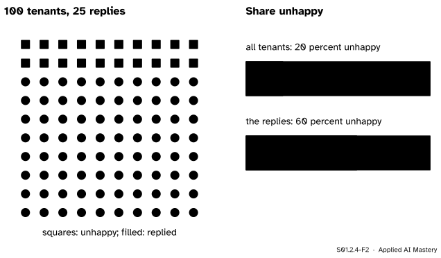
A volunteer sample lets the units choose themselves. A landlord with 100 tenants, 20 of them unhappy with their rent, invites comments. Fifteen of the 20 unhappy tenants reply and 10 of the 80 content ones do.
S01.2.4-F2
A volunteer sample. Unhappy tenants reply far more often than content ones, so 60 percent of the replies are unhappy while only 20 percent of the tenants are.
The replies are \(15 / 25 = 60\) percent unhappy; the tenants are \(20 / 100 = 20\) percent unhappy. Online reviews work the same way: people with strong views write them.
A frame that leaves units out. The website without Centre of lesson S01.2.2 centres on 6.125 however many flats it lists.
Non-response. The units were chosen fairly, but some do not answer. Ten flats are asked, with rents 4, 5, 6, 7, 8, 9, 10, 12, 15 and 24: they add to 100, a mean of 10. The three dearest decline to say, and the seven answers average \(49 / 7 = 7\). The Literary Digest poll of lesson S01.2.2 got ballots back from only about a quarter of the people it wrote to, and those who did not reply leaned heavily towards Roosevelt.
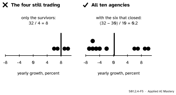
Survivorship. Only the units that lasted are there to be counted. Ten letting agencies opened in 2015. The four still trading report yearly growth of 6, 7, 9 and 10 percent, a mean of 8. The six that closed had averaged \(-5\) percent before they shut, and they are in no table. All ten together grew by \({(32 - 30) / 10} = 0.2\) percent a year.
The formal statement
Two results explain most of these cases.
Asking members instead of groups. Suppose there are \(G\) groups (classes, buildings, households) of sizes \(n_1, \dots, n_G\), with \(n = n_1 + \cdots + n_G\) members in all. Ask every group its size and average: you get the plain mean \(\frac{1}{G}\sum_g n_g\). Now ask every member the size of their own group. The \(n_g\) members of group \(g\) all answer \(n_g\), so their answers add to \({n_g \cdot n_g}\), and the average over all \(n\) members is
The middle form is the weighted mean of lesson S01.2.3 with each group weighted by its share of the members, \(n_g / n\), instead of by one over \(G\). Big groups get big weights, so the member average is larger, and it equals the group average only when all groups are the same size (the deeper block below proves it). This is size-biased sampling. It is not an error in either average; they answer two different questions, and the error is to quote one as the other.
Selection that depends on the value. Suppose unit \(i\), with value \(x_i\), gets into the table with chance \(p_i\). Ask the whole population many times over and pool every answer. Unit \(i\) answers in a share \(p_i\) of the askings, so in the pool it appears in proportion to \(p_i\), and the pooled answers average
This is again a weighted mean, now with weights \(p_i\). If every \(p_i\) is the same, the weights cancel and the answers average \(\mu\). If \(p_i\) falls as \(x_i\) rises, the large values get the small weights and the answers average below \(\mu\), at every sample size, because the weights do not depend on \(n\).
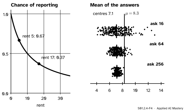
For the city, let a flat report its rent with chance \(10 / {(10 + \text{rent})}\): a flat at 10 reports half the time, one at 5 two times in three, one at 17 about three times in eight. The weighted mean comes to 7.13, against \(\ctruth{\mu} = 8.3\).
S01.2.4-F4
Selection on the outcome. Left: the dearer the flat, the less likely its rent is reported. Right: ask 16, 64 or 256 flats, 1,000 times each: the answers scatter less as more are asked, but they centre near 7.1 every time.
Go deeper: the member average is never below the group average
Write \(\bar{n} = \frac{1}{G}\sum_g n_g\) for the group average, so that \(\sum_g n_g = G\bar{n}\). A sum of squares cannot be negative, so
The second line expands each square, the third uses \(\sum_g n_g = G\bar{n}\). So \(\sum_g n_g^2 \ge G\bar{n}^2 = \bar{n} \sum_g n_g\), and dividing by \(\sum_g n_g\) gives member average \(\ge \bar{n}\). Equality needs every \(n_g - \bar{n} = 0\): all groups the same size.
The same algebra explains a trick for selection on the value. If the chances \(p_i\) were known, weighting each answer by \(1 / p_i\) would cancel them:
Survey weighting rests on this idea. The catch is that when the chance depends on the missing value itself, nobody knows \(p_i\).
Worked example
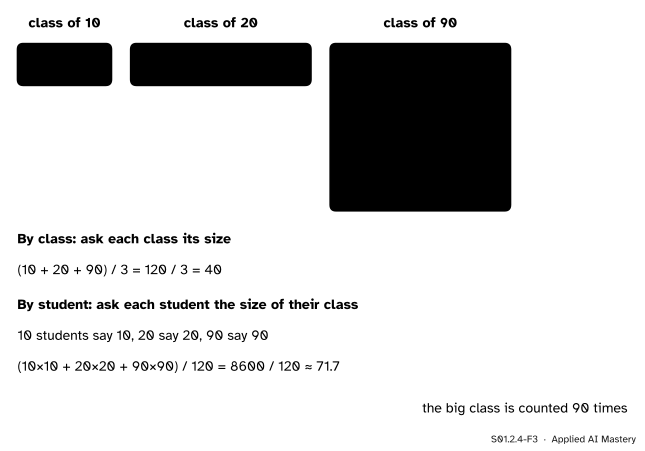
Classes of 10, 20 and 90. A department runs three classes. The department reports its average class size; a survey asks students how big their class is.
S01.2.4-F3
One department, two averages. By class it is 40; by student it is about 71.7, because the class of 90 is reported by 90 students.
By class.\({(10 + 20 + 90) / 3} = 120 / 3 = 40\).
By student. Ten students answer 10, twenty answer 20 and ninety answer 90. The answers add to \({10 \cdot 10} + {20 \cdot 20} + {90 \cdot 90} = 100 + 400 + 8100 = 8600\), over 120 students:
\[
\frac{8600}{120} \approx 71.7 .
\]
As weights: the classes’ shares of the students are \(10/120\), \(20/120\) and \(90/120\), so the class of 90 carries three quarters of the weight. Both numbers are true. The department’s 40 answers “how big is a class?”; the students’ 71.7 answers “how big is the class a student sits in?”. Each is wrong as an answer to the other question.
Code
The class sizes from scratch, then as a weighted mean with numpy.average.
import numpy as npimport pandas as pdsizes = [10, 20, 90]by_class =sum(sizes) /len(sizes)answers = [s for s in sizes for _ inrange(s)] # every student reports their class's sizeby_student =sum(answers) /len(answers)print("by class:", by_class, " by student:", round(by_student, 2)," formula:", round(sum(s * s for s in sizes) /sum(sizes), 2))print("as a weighted mean:", round(np.average(sizes, weights=sizes), 2))
by class: 40.0   by student: 71.67   formula: 71.67
as a weighted mean: 71.67
Now selection on the outcome in the city, built as in every lesson of the course. Ask \(n\) flats by lot, let each report its rent with chance \(10 / {(10 + \text{rent})}\), and average what comes back.
rng = np.random.default_rng(0)n_flats = {"South": 250, "North": 150, "Centre": 100}district_mean = {"South": 5, "North": 8, "Centre": 17}rents, district = [], []for name in ("South", "North", "Centre"): draws = rng.gamma(9.0, 1.0, n_flats[name]) rents.append(draws * district_mean[name] / draws.mean()) district += [name] * n_flats[name]rents, district = np.concatenate(rents), np.array(district)mu = rents.mean()p =10/ (10+ rents)pooled = (p * rents).sum() / p.sum()print(f"mu = {mu:.2f}, weighted mean of the answers = {pooled:.2f}")rng = np.random.default_rng(1)centres = {}for n in (16, 64, 256): means = []for _ inrange(1000): asked = rng.choice(len(rents), n, replace=False) told = asked[rng.random(n) < p[asked]]iflen(told): means.append(rents[told].mean()) centres[n] = np.mean(means)print(f"ask {n:3d}: the answers centre on {centres[n]:.2f}")
mu = 8.30, weighted mean of the answers = 7.13
ask  16: the answers centre on 7.07
ask  64: the answers centre on 7.11
ask 256: the answers centre on 7.14
At every \(n\) the centre sits near 7.1, more than a whole unit below \(\mu\): the number the website announced. What can the table itself reveal? Not the missing rents. But the asked flats have other columns, such as the district, and comparing those who answered with those who did not is the first check to run.
Centre’s flats answer least often. That does not prove the rents are biased, but it shows the answers are not a simple random sample of the asked flats, and it points at the dear end of the city.
Explore
This module’s interactive, the sampling bench, lives in lesson S01.2.2. Its method dear flats answer more is selection on the outcome running the other way: there the answers centre above \(\mu\). Try every sample size and watch the centre refuse to move.
Pitfalls
S01.2.4-F5
Wrong beside right. Averaging the agencies still trading gives 8 percent a year; counting the six that closed gives 0.2 percent.
“The table is the data; I can only analyse what is in it.”
You can also ask what is not in it. Before any summary or model, put two questions to the table: who is missing, and why? A table of current customers has no one who left; a table of approved loans has no repayment record for anyone refused. A model trained on such rows learns about the survivors (sources of bias, R01.2).
“With enough responses the bias averages out.”
Bias from selection does not shrink with \(n\). The city’s answers centre near 7.1 whether 16 or 256 flats are asked. The Literary Digest had 2.4 million replies.
“Reweighting by district fixes non-response.”
Weighting by district (lesson S01.2.3) repairs selection that depends on the district alone. Here the dear flats inside every district answer less often, so the answers are too low within each district too, and no district weight can see that. Lesson S01.6.2 names the two cases MAR and MNAR.
Check yourself
Recall
1. Name the five doors of this lesson by which a sample can go wrong.
Show answer
Convenience, volunteering, a frame that leaves units out, non-response, and survivorship.
2. Classes have sizes 10, 20 and 90. What do the class average and the student average come to?
Show answer
40 by class, and \(8600 / 120 \approx 71.7\) by student.
3. Write the average that comes from asking members about the size of their group.
Show answer
\(\sum_g n_g^2 / \sum_g n_g\): each group’s size weighted by its share of the members.
4. If unit \(i\) answers with chance \(p_i\), what do the pooled answers average, and when is it below \(\mu\)?
Show answer
\(\sum_i p_i x_i / \sum_i p_i\). It is below \(\mu\) when the chance of answering falls as the value rises.
5. What two questions should you put to any data set before modelling it?
Show answer
Who is missing, and why?
Exercises
1.★ A school has four classes of 15, 15, 30 and 60 students. Find the average class size by class and by student.
Show solution
By class: \({(15 + 15 + 30 + 60) / 4} = {120 / 4} = 30\). By student:
2.★★ Of 200 tenants, 50 pay more than 10 (mean 15) and 150 pay at most 10 (mean 6). A survey reaches all of them; 20 percent of the first group answer and 60 percent of the second. Find \(\mu\) and the mean of the answers, and check it against the weighted-mean formula.
Show solution
\(\mu = {({50 \cdot 15} + {150 \cdot 6}) / 200} = {(750 + 900) / 200} = 8.25\). The answers come from \({0.2 \cdot 50} = 10\) dear tenants and \({0.6 \cdot 150} = 90\) others, so they average \({({10 \cdot 15} + {90 \cdot 6}) / 100} = {(150 + 540) / 100} = 6.9\). With the formula, each dear tenant has \(p = 0.2\) and each other \(p = 0.6\):
3.★★★ Three buildings hold 4, 6 and 20 flats. (a) Find the mean building size and the mean size of the building a flat is in. (b) Without the deeper block, explain in words why the second can never be smaller than the first.
(b) The by-flat average is a weighted mean of the same three sizes, with weights proportional to the sizes themselves. Moving weight from small values onto large ones can only raise a mean, and it raises it not at all only when there is nothing to move: when all buildings have the same size.
Summary card
Who is missing, and why? The answer decides what the table can tell you.
S01.2.4-F1
Each door bends the mean.
Doors: convenience, volunteering, the frame, non-response, survivorship.
Asking members, not groups:\(\sum_g n_g^2 / \sum_g n_g \ge\) the group average.
Chance \(p_i\) of getting in: answers average \(\sum_i p_i x_i / \sum_i p_i\), at every \(n\).
More rows shrink the scatter, never this bias.
Sources and next steps
Sources. Each was opened and checked against this lesson on 12 November 2026.
David Diez, Mine Cetinkaya-Rundel and Christopher Barr, OpenIntro Statistics, 4th edition, Section 1.3.3: non-response bias (if only 30 percent of those sampled respond, the results may not represent the population), convenience samples, and ratings written only by people who go out of their way to give one.
Barbara Illowsky and Susan Dean, Introductory Statistics 2e, OpenStax, Section 1.2: convenience sampling uses results that are readily available, and sampling bias leads to wrong conclusions about the population.
Allen B. Downey, Think Stats, 3rd edition, Section 3.3, “The Class Size Paradox”: a small class has few students and a large class many, so when students are asked, the chance of observing a class is proportional to its size.
Next. Module S01.3, Center, spread and shape, studies the mean and its relatives as numbers in their own right, now that the nine flats are known to be a sample. Missing cells, rather than missing rows, are module S01.6, and dataset shift in machine learning is E05.4.