Stone size steers both the choice of operation and its chance of success. Name such a confounder, compare like with like by stratifying, compute one fair figure by direct standardisation, and list the rivals to any causal reading of a correlation.
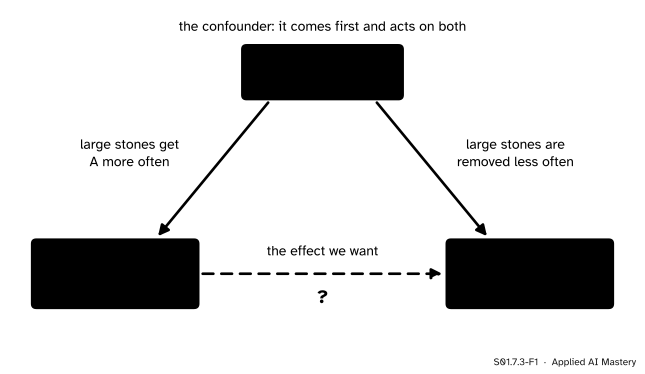
Define a confounder as a variable that influences both the thing being compared and the outcome, and draw it as a fork of three boxes.
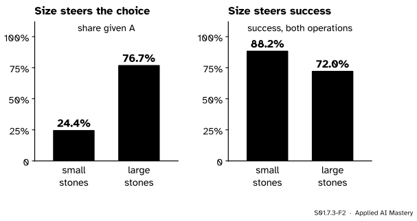
Measure both arrows of the fork in a table: how the confounder steers the choice and how it steers the outcome.
Compute directly standardised rates by applying each treatment’s group rates to one shared mix, and show that their difference is a weighted mean of the group differences.
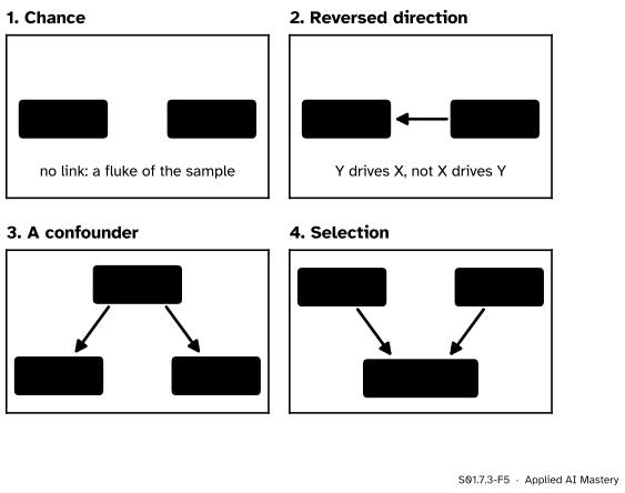
List the rival explanations of an association (chance, reversed direction, a confounder, selection) before reading it as a cause.
In review. The maths and code on this page are checked by automated tests on every change, but an independent reader has not signed it off yet. Spot a mistake or a confusing step? Tell us.
The question
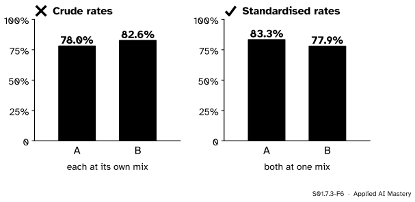
Across all 700 kidney-stone patients, the keyhole operation B succeeded more often than open surgery A: 82.6% against 78.0%. Inside each stone size, A did better. If you had to report one number per operation that compares them fairly, what would it be, and what is the third variable that made the raw comparison unfair?
From the last lesson
1. For the eight study points, how does the pooled sum of products of −34 split?
Show answer
Into \(+6\) within the two courses (\(+3\) each) and \(-40\) between them (\(-20\) for each course mean).
2. When does a trend that rises inside every group fall when the groups are pooled?
Show answer
When the group means line up against the trend and the between part outweighs the within part, \(B < -W\).
Intuition
In both lessons so far a third variable did the damage: stone size in the table, the course in the scatter plot. It is worth naming what that variable does.
S01.7.3-F1
Stone size is a confounder. It has an arrow into the treatment and an arrow into success, so the raw link between treatment and success mixes the effect we want with the effect of stone size.
The arrows say “influences”. Stone size influences which operation a doctor chooses: large stones get open surgery more often. Stone size also influences success: large stones are harder to remove, whichever operation is used. A variable with both arrows is called a confounder, because it confounds (mixes together) two effects. The comparison of A with B picks up the effect of the operation and the effect of stone size, since the two operations were given to different mixes of stones.
The shape of the picture, one box with arrows to two others, is called a fork. Course S06 studies forks and other causal diagrams properly; here one picture is enough.
The cure follows from the picture. If stone size is what differs between the two groups of patients, compare patients with the same stone size. That is stratifying: splitting the data into groups, or strata, inside which the confounder does not vary.
Build it up
Step 1. Measure the arrow into the treatment. Of the 357 patients with small stones, 87 got A: 24.4%. Of the 343 with large stones, 263 got A: 76.7%. Stone size steered the choice strongly.
Step 2. Measure the arrow into success. For both operations together, 315 of the 357 small stones were removed successfully (88.2%) and 247 of the 343 large ones (72.0%). Stone size steered success too.
S01.7.3-F2
The two arrows of the fork, measured in the table. Large stones were far more likely to get A, and far less likely to be removed successfully.
Step 3. Stratify. Inside the small stones, A beats B by 6.4 points (93.1% against 86.7%). Inside the large stones, A beats B by 4.3 points (73.00% against 68.75% before rounding). Inside each stratum, stone size cannot explain the difference, because it does not vary there.
Step 4. Ask for one number. Two differences, 6.4 and 4.3, are honest but awkward to report. One figure per operation would be easier, as long as it compares the operations on the same patients. The next section builds it.
Step 5. Keep the rivals in mind. Stone size is one reason why a raw association can mislead. A careful reader checks for four, drawn below, before reading any association between X and Y as “X causes Y”.
S01.7.3-F5
Four rival explanations of an association between X and Y. Each can produce an association with no arrow from X to Y at all.
Chance. In a small sample, or when many pairs of columns are searched, some correlations are large by luck alone. Irizarry’s chapter shows unrelated columns of 25 values whose largest correlation, out of a million tries, reaches 0.83. Course S02 measures how large luck can make an association.
Reversed direction. Y may drive X. Patients who are more ill are given more treatment, so treatment and illness go together because illness causes treatment.
A confounder. A third variable Z may drive both, as stone size does here.
Selection. If whether a row gets into the table depends on X and on Y, the rows that remain can show an association that the whole population does not have. This is the selection of S01.2.4, now acting on two columns at once; S06 studies it.
“Correlation is not causation” is the short form of this list. An association is a fact about the table; a cause is a claim about what would happen if you changed X, and every rival must be ruled out before the second follows from the first.
The formal statement
NoteDefinition: confounder (first look)
A confounder of a comparison of treatments is a variable that comes before the treatment, that influences which treatment a unit gets, and that influences the outcome by itself.
Course S06 replaces this with a definition in terms of causal diagrams. At this level the three conditions are enough to recognise the trap.
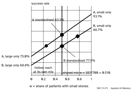
Direct standardisation. Let the strata be \(g = 1, 2\) and let treatment A have group rates \(p_g^{\text{A}}\), treatment B \(p_g^{\text{B}}\). Choose one standard mix: shares \(\cparam{W_g}\), not negative and adding to 1. The usual choice is the mix of all the units together, here \(\cparam{W_1} = 357/700\) small and \(\cparam{W_2} = 343/700\) large. The directly standardised rate of a treatment is its group rates averaged with the standard weights:
It is the weighted mean of S01.2.3 and S01.7.1, with one change: the weights are the same for both treatments. Each standardised rate answers the question “what would this treatment’s success rate be on the standard mix of patients?”.
The standardised difference is a weighted mean of the group differences. Subtract the two lines and collect the terms of each stratum:
So the standardised comparison is built only from comparisons inside the strata, which stone size cannot bias. If A is ahead in every stratum, it is ahead after standardising, whatever standard mix is chosen; this is the “one shared mix” result of S01.7.1 again.
S01.7.3-F3
Direct standardisation reads both treatments’ lines at one shared mix (orange). The crude rates (hollow) sit at two different mixes; the standardised rates sit one above the other.
Go deeper: standardising with a different standard mix
The standard mix is a choice, and a different choice gives different standardised rates. With A’s own mix (24.9% small) as the standard, A keeps its 78.0% and B gets \({0.2486 \times 0.8667} + {0.7514 \times 0.6875} = 0.732\), so A leads by 4.8 points. With B’s mix (77.1% small), B keeps its 82.6% and A gets \({0.7714 \times 0.9310} + {0.2286 \times 0.7300} = 0.885\), a lead of 5.9 points. The size of the lead depends on the mix, because the two strata differences, 6.4 and 4.3 points, are not equal; the lead always lies between them. Report the standard mix with a standardised rate, as you would report the unit of a measurement.
Worked example
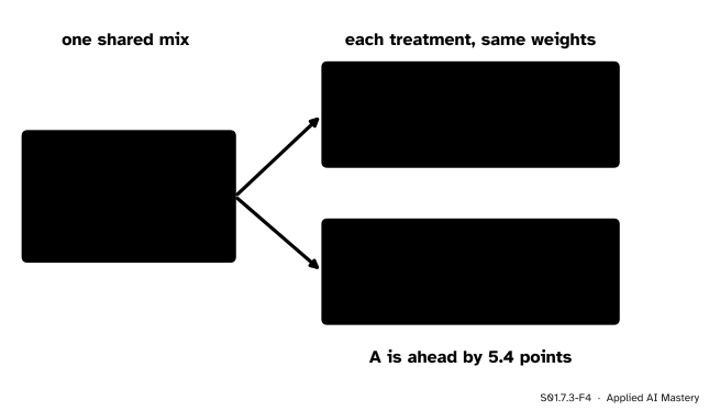
Standardise both operations to the mix of all 700 patients.
S01.7.3-F4
The trace of the worked example: one set of weights, used twice.
The standard weights. All 700 patients: 87 + 270 = 357 had small stones and 263 + 80 = 343 had large ones. So \(W_1 = 357/700 = 0.510\) and \(W_2 = 343/700 = 0.490\).
On the same mix of patients, A succeeds 83.3% of the time and B 77.9%: A is ahead by 5.4 points. Check with the group differences, 6.44 and 4.25 points before rounding: \({0.510 \times 6.44} + {0.490 \times 4.25} = 5.37\), which is 5.4 points, a weighted mean of the two stratum differences, as the formula said. The crude comparison had B ahead by 4.6 points; standardising has removed the part of the gap that came from the mix of stones.
Code
First from scratch: a weighted mean as a sum of products over a sum of weights, used once per treatment with the same weights.
rates = {"A": {"small": 81/87, "large": 192/263},"B": {"small": 234/270, "large": 55/80}}standard = {"small": 87+270, "large": 263+80} # all 700 patients: the standard mixdef weighted_mean(values, weights): total =sum(weights.values())returnsum(weights[k] * values[k] for k in weights) / totalstd = {t: weighted_mean(rates[t], standard) for t in rates}gaps = {k: rates["A"][k] - rates["B"][k] for k in standard}print({t: round(100* v, 1) for t, v in std.items()})print("lead of A:", round(100* (std["A"] - std["B"]), 1)," from the gaps:", round(100* weighted_mean(gaps, standard), 1))
{'A': 83.3, 'B': 77.9}
lead of A: 5.4  from the gaps: 5.4
Now with numpy.average, whose weights argument does the division by the sum of the weights for us. The other two standard mixes of the deeper block come out of the same call.
import numpy as nporder = ["small", "large"]mixes = {"all 700": [357, 343], "A's own mix": [87, 263], "B's own mix": [270, 80]}for name, weights in mixes.items(): a = np.average([rates["A"][k] for k in order], weights=weights) b = np.average([rates["B"][k] for k in order], weights=weights)print(f"{name:12s} A {100* a:.1f}% B {100* b:.1f}% lead of A {100* (a - b):.1f}")
all 700       A 83.3%  B 77.9%  lead of A 5.4
A's own mix   A 78.0%  B 73.2%  lead of A 4.8
B's own mix   A 88.5%  B 82.6%  lead of A 5.9
With A’s own mix, A keeps its crude 78.0% and B drops to 73.2%; with B’s own mix, B keeps its crude 82.6% and A rises to 88.5%. Whatever the shared mix, A is ahead.
Explore
The module’s interactive, Split the scatter, is in S01.7.2. Read it now as a picture of a confounder: the course is the third variable. It shifts the hours (advanced students study more) and it shifts the scores (its test is harder). Set both gaps to zero and the course no longer acts on either axis; the pooled line then runs like the lines inside the courses, as if the confounder had been removed.
Pitfalls
S01.7.3-F6
Wrong beside right. Crude rates compare two operations on two different mixes of patients; standardised rates compare them on one.
“Adjusting for a variable always gives the true effect.”
Standardising removes the part of a gap that comes from the variables you stratified by, and nothing else. If another confounder was never recorded (how experienced the surgeon was, say), the standardised rates still carry its effect. A table can only be adjusted for the columns it has.
“The standardised rate is what the hospital actually achieved.”
It is a counterfactual summary: the rate the treatment would have had on the standard mix. A’s real patients succeeded 78.0% of the time. Report crude and standardised rates side by side, and name the standard mix.
“A strong association in a large data set must be a cause.”
Size helps only with the first rival, chance. A confounder, a reversed direction or a selection rule produces an association that does not shrink with more rows. In machine learning this is how a model learns a shortcut: a feature that merely travels with the label, because of a third variable behind both, predicts well until the third variable changes (S01.7.4).
Check yourself
Recall
1. State the three conditions of a confounder at this level.
Show answer
It comes before the treatment, it influences which treatment a unit gets, and it influences the outcome by itself.
2. How did stone size steer the choice of operation and the chance of success?
Show answer
24.4% of small stones but 76.7% of large stones got A; 88.2% of small stones but 72.0% of large stones were removed successfully.
3. What is a directly standardised rate?
Show answer
A treatment’s group rates averaged with one standard set of weights, \(\sum_g W_g p_g\), the same weights for every treatment.
4. What are the standardised rates of A and B on the mix of all 700 patients?
Show answer
83.3% for A and 77.9% for B, a lead of 5.4 points for A.
5. Name the four rival explanations of an association.
Show answer
Chance, reversed direction, a confounder, and selection.
Exercises
1.★ In exercise 1 of S01.7.1, hospital P had mild 95/100 and severe 120/300, and hospital Q had mild 270/300 and severe 35/100. Standardise both to the combined mix of their 800 patients.
Show solution
The combined mix is \(100 + 300 = 400\) mild and \(300 + 100 = 400\) severe, so \(W_1 = W_2 = 0.5\). P: \({0.5 \times 0.95} + {0.5 \times 0.40} = 0.675\). Q: \({0.5 \times 0.90} + {0.5 \times 0.35} = 0.625\). On the same patients P is ahead by 5 points, although its crude rate (53.75%) was far below Q’s (76.25%).
2.★★ Which rival explanation fits each claim best? (a) An analyst checks all 190 pairs among 20 columns and reports the strongest correlation. (b) People who take more painkillers report more pain. (c) Ice-cream sales and drownings rise and fall together over a year. (d) Among films that won an award, the longer ones have lower box-office takings.
Show solution
(a) Chance: the largest of 190 correlations is large by luck even if no pair is related. (b) Reversed direction: pain drives the painkillers. (c) A confounder: hot weather drives both. (d) Selection: a film gets into the table by winning, which can depend on its length and on its takings, so the association inside the table need not hold for all films.
3.★★★ Prove that the directly standardised difference \({p_{\text{std}}^{\text{A}} - p_{\text{std}}^{\text{B}}}\) always lies between the smallest and the largest stratum difference \({p_g^{\text{A}} - p_g^{\text{B}}}\), for any standard mix and any number of strata. Check it for the kidney stones with the three mixes of the Code section.
Show solution
Write \(d_g = {p_g^{\text{A}} - p_g^{\text{B}}}\). Subtracting the two standardised rates and collecting the terms of each stratum gives \({\sum_g W_g p_g^{\text{A}} - \sum_g W_g p_g^{\text{B}}} = \sum_g W_g d_g\). The weights are not negative and add to 1, so this is a weighted mean of the \(d_g\). By the argument of exercise 3 in S01.7.1, with \(m\) the smallest and \(M\) the largest \(d_g\), each \(W_g d_g\) lies between \(W_g m\) and \(W_g M\), and adding gives \(m \le \sum_g W_g d_g \le M\). For the kidney stones \(d_1 = 6.4\) and \(d_2 = 4.3\) points, and the three standardised leads, 5.4, 4.8 and 5.9 points, all lie between 4.3 and 6.4.
Summary card
A confounder acts on both the treatment and the outcome; compare like with like.
S01.7.3-F1
The fork: one variable behind both.
Confounder. Comes first, steers the treatment, steers the outcome.
Stratify. Compare treatments inside groups where the confounder does not vary.
Standardise.\(p_{\text{std}} = \sum_g W_g p_g\) with one shared mix: 83.3% for A, 77.9% for B.
Rivals. Chance, reversed direction, a confounder, selection.
Sources and next steps
Sources. Each was opened and checked against this lesson on 12 November 2026.
Judea Pearl, Madelyn Glymour and Nicholas P. Jewell, Causal Inference in Statistics: A Primer, chapter 1 (the authors’ copy). Section 1.2 explains the reversal by a common cause of drug taking and recovery, concludes that subjects of the same kind must be compared, and recalls that correlation is not causation.
Rafael A. Irizarry, Introduction to Data Science, chapter 19, Association is not causation: spurious correlation (a largest correlation of 0.83 among a million groups of 25 unrelated pairs), outliers, reversing cause and effect, and confounders, with stratifying as the remedy.
NumPy documentation, numpy.average: the weighted average, the sum of the weights times the values divided by the sum of the weights.