Anomalies are few and different, so random cuts fence them off quickly. Grow isolation trees, measure path lengths, derive the normaliser c(n) as the average path of an unsuccessful search in a binary search tree, and score points with Liu, Ting and Zhou’s s = 2^(-E[h]/c(n)).
ML03.9.3L2 Intermediate30 minIn review (what this means)
The maths and code on this page are checked by automated tests on every change, but an independent reader has not signed it off yet. Spot a mistake or a confusing step? Tell us.
Grow an isolation tree by random cuts and read a point’s path length h(x) from it.
Derive the normaliser c(n) = 2 H(n - 1) - 2(n - 1)/n from a recurrence, and compute c(256) = 10.245.
Turn average path lengths into the anomaly score s = 2^(-E[h(x)]/c(n)) and read its three limits.
Explain why each tree is grown on a small subsample of 256 points.
Build an isolation forest from scratch on the twelve points and use sklearn.ensemble.IsolationForest with score_samples and contamination.
The question
The Mahalanobis distance needs a covariance, and the local outlier factor needs every point’s nearest neighbours: for a million card payments, that is a lot of distances. Yet anomalies are few and different. If you cut the data at random, a point standing on its own should be fenced off after only a few cuts, while a point in a crowd needs many. Can counting random cuts, with no distance measured at all, find the anomalies?
From the last lesson
1. What does the local outlier factor compare?
Show answer
A point’s local reachability density with the mean density of its \(k\) nearest neighbours. A value near 1 means “as crowded as my neighbours”; a large value means “much sparser”.
2. Why can a small \(k\) hide a clump of anomalies from LOF?
Show answer
If \(k\) is smaller than the clump, each of its points finds all its neighbours inside the clump, so its density matches theirs and its LOF is close to 1.
Intuition
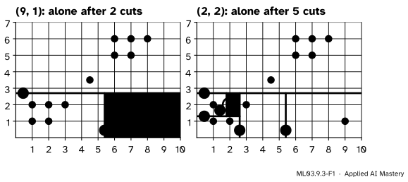
Pick a feature at random, then a threshold at random between that feature’s smallest and largest value, and cut. Repeat inside each piece. A point that stands alone is fenced off after a few cuts; a point in a crowd needs many.
ML03.9.3-F1
The same random tree, read for two points. The far point \((9, 1)\) is alone after 2 cuts; the corner \((2, 2)\) of the lower group needs 5.
The number of cuts it takes to isolate a point is its path length. Short paths mean strange points. This is the isolation forest of Liu, Ting and Zhou (2008). It never measures a distance, which makes it fast, and it builds only the shallow part of each tree, because that is where the anomalies are isolated.
Build it up
Step 1. One isolation tree. Start with all points in one node. While a node holds more than one point, choose a feature at random, and a threshold uniformly between that feature’s minimum and maximum in the node. Points below the threshold go left, the rest go right. A cut is the same kind of test as in a decision tree (ML02.1), but it is chosen at random, with no labels and no impurity.
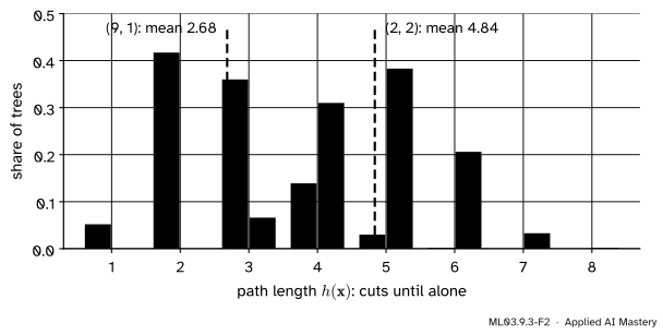
Step 2. Many trees. One tree is a lottery: a lucky first cut can isolate the far point at once, or a normal point early. Grow many trees and average each point’s path length.
ML03.9.3-F2
Path lengths of two points over 1000 random trees grown to full depth. The far point averages 2.68 cuts; the corner \((2, 2)\) averages 4.84.
Step 3. A yardstick. Is an average path of 2.68 short? That depends on how many points the tree holds: more points means deeper trees for everybody. So divide by the average path a point would need in a tree of \(n\) points, \(c(n)\), derived below.
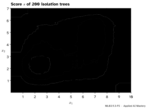
Step 4. A score over the plane. Pass every location of the plane through the trees and shade it by its score. The picture shows where the forest thinks anomalies live.
ML03.9.3-F5
The score of 200 trees over the plane. It is low inside the blobs and high near the edges. Its contours run along the axes, because every cut does; the stray between the blobs is not in the top 3.
The formal statement
NoteDefinitions: isolation tree and path length
An isolation tree on a set of points is either a leaf, or a test \({x_q < p}\) on one feature \(q\) with two subtrees for the points that pass and fail it (Liu et al., section 2). The path length\(h(\vect{x})\) is the number of edges from the root to the leaf where \(\vect{x}\) ends.
The normaliser. Liu et al. borrow it from binary search trees: in a tree built from \(n\) points where every cut is equally likely to fall in each of the \(n - 1\) gaps between neighbouring values, let \(a(n)\) be the expected sum of the depths of all \(n\) leaves. At the root every point moves one level down, adding \(n\); then the two sides hold \(i\) and \(n - i\) points:
with \(a(1) = 0\); the two sums are equal because \(i\) and \(n - i\) run over the same values. Write \({S_m = a(1) + \dots + a(m)}\). Multiply by \(n - 1\), and write the same equation for \(n + 1\):
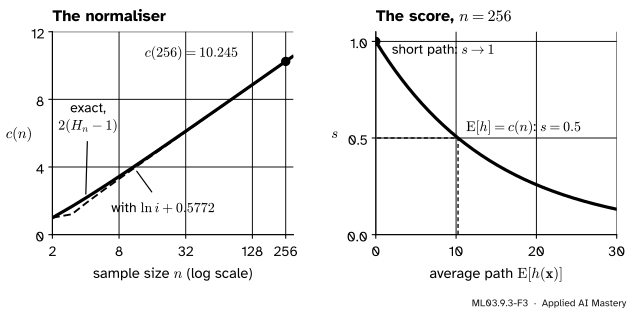
where the last step uses \({H(n) = H(n-1) + 1/n}\), so that \({2/n - 2 = -2(n-1)/n}\). This is equation (1) of the paper, the average path length of an unsuccessful search in a binary search tree. In practice \({H(i) \approx \ln i + 0.5772}\) (Euler’s constant), which gives \({c(256) = 10.245}\) and \({c(8) = 3.296}\); the exact sums give 10.249 and 3.436. scikit-learn uses the estimate.
NoteResult: the anomaly score
With \(\E[h(\vect{x})]\) the average path length over the trees, each grown on \(n\) points,
Read its limits from the exponent. If \({\E[h] \to 0}\) then \({s \to 2^0 = 1}\): definitely an anomaly. If \({\E[h] = c(n)}\) then \({s = 2^{-1} = 0.5}\): a typical point. If \({\E[h] \to n - 1}\), the deepest possible, then \(s\) is near 0. The paper’s rule of thumb: \(s\) close to 1 is an anomaly, \(s\) well below 0.5 is normal, and if every point scores about 0.5 there is no clear anomaly.
ML03.9.3-F3
Left: the normaliser grows like \(2\ln n\). Right: the score turns an average path into a number in \((0, 1]\), with 0.5 exactly at the average path \(c(n)\).
Subsampling and the height limit. Each tree is grown on a random subsample of \(\psi\) points, 256 by default, and stops at height \({\lceil \log_2 \psi \rceil}\), about the average tree height (section 4.1). A leaf that still holds several points adds \(c(\text{size})\) to the path, an estimate of the depth the unbuilt subtree would add (Algorithm 3). The forest has \(t = 100\) trees by default; the paper finds path lengths usually settle well before that.
Worked example
One tree on the twelve points, by hand. Suppose the random draws give these six cuts, each inside its node’s range:
ML03.9.3-F4
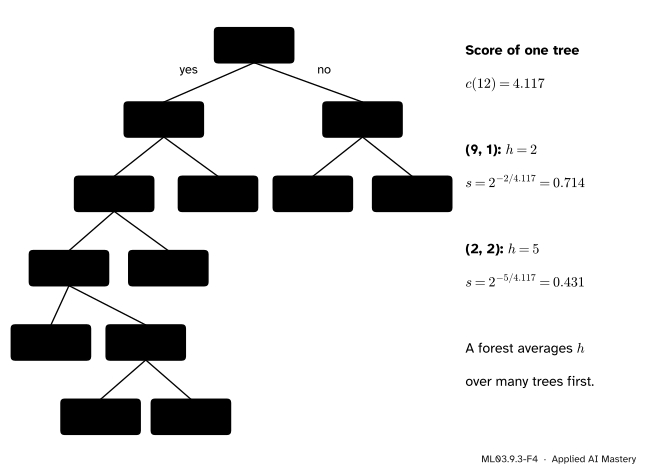
The hand-drawn tree of the anchor figure. Anomalies end in shallow leaves (reddish purple); normal points in deep ones (blue).
Cut 1, on \(x_2\) at 2.7 (the range is 1 to 6), sends the five lower points and \((9, 1)\) left and the rest right. Cut 2, on \(x_1\) at 5.4 (range 1 to 9), leaves \((9, 1)\) alone: \({h(9, 1) = 2}\). Cut 3, on \(x_1\) at 5.1 (range 4.5 to 8), leaves the bridge alone: \({h = 2}\). Cuts 4, 5 and 6, at \({x_1 = 2.6}\), \({x_2 = 1.3}\) and \({x_1 = 1.8}\), peel off \((3, 2)\) at depth 3 and finally \((1, 2)\) and \((2, 2)\) at depth 5.
Scores from this one tree. With all twelve points,
The far point gets \({2^{-2/4.117} = 0.714}\) and \((2, 2)\) gets \({2^{-5/4.117} = 0.431}\).
Result: in this tree the anomalies sit at depth 2 and the corner of the square at depth 5. A forest averages such depths over many random trees, as the code does next.
Code
From scratch: the paper’s tree (Algorithm 2), grown to full depth, and the path length with the \(c(\text{size})\) adjustment at a leaf (Algorithm 3).
import mathimport numpy as npX = np.array([(1, 1), (2, 1), (1, 2), (2, 2), (3, 2), (6, 5), (7, 5), (6, 6), (7, 6), (8, 6), (4.5, 3.5), (9, 1)], dtype=float)def c(n):if n <=1:return0.0if n ==2:return1.0return2* (math.log(n -1) +0.5772156649) -2* (n -1) / ndef grow(idx, rng):iflen(idx) <=1:return ("leaf", len(idx)) sub = X[idx] spread = [f for f inrange(X.shape[1]) if sub[:, f].max() > sub[:, f].min()]ifnot spread:return ("leaf", len(idx)) f = spread[rng.integers(len(spread))] t = rng.uniform(sub[:, f].min(), sub[:, f].max())return ("node", f, t, grow(idx[X[idx, f] < t], rng), grow(idx[X[idx, f] >= t], rng))def path(tree, x, depth=0):if tree[0] =="leaf":return depth + c(tree[1]) _, f, t, left, right = treereturn path(left if x[f] < t else right, x, depth +1)rng = np.random.default_rng(0)forest = [grow(np.arange(len(X)), rng) for _ inrange(1000)]Eh = np.array([np.mean([path(T, x) for T in forest]) for x in X])s =2** (-Eh / c(len(X)))order = np.argsort(-s)print("c(12), c(256):", round(c(12), 3), round(c(256), 3))print("E[h] of (9, 1), bridge, (2, 2):", Eh[[11, 10, 3]].round(2))print("top three:", X[order[:3]].tolist(), s[order[:3]].round(3))
The far point and the bridge come first, about 0.64 and 0.55. But the corner \((8, 6)\) is close behind the bridge: a point at the edge of the range is easy to cut off too.
scikit-learn’s score_samples returns \(-s\). With contamination="auto" it flags every point with \({s > 0.5}\); with a number, it flags that share of the training points.
from sklearn.ensemble import IsolationForestauto = IsolationForest(random_state=0).fit(X)sk =-auto.score_samples(X)two = IsolationForest(random_state=0, contamination=2/12).fit(X)print("max_samples used:", auto.max_samples_, " offset_:", auto.offset_)print("top two by s:", X[np.argsort(-sk)[:2]].tolist(), np.sort(sk)[::-1][:2].round(3))print("auto flags", int((auto.predict(X) ==-1).sum()), "points; contamination 2/12 flags", X[two.predict(X) ==-1].tolist())
max_samples used: 12  offset_: -0.5
top two by s: [[9.0, 1.0], [4.5, 3.5]] [0.634 0.555]
auto flags 5 points; contamination 2/12 flags [[4.5, 3.5], [9.0, 1.0]]
With only twelve points the default flags five, every point with \({s > 0.5}\). Give the contamination you expect, or rank.
Explore
ML03.9-X1
Isolation forest explorer
Press Split to cut the box around the chosen point (the large one) until it stands alone, and count the cuts. Then drag it, or move it with the sliders, from inside a blob to a corner and compare. Press Grow 50 trees to shade the score over the plane, and slide the contamination to flag the top points.
Try the point in the gap between the blobs: it is strange to a density, but random cuts often take several steps to fence it off, because it sits in the middle of the range of both features.
Pitfalls
ML03.9.3-F6
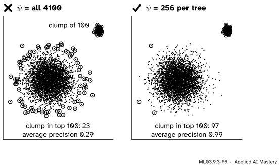
Wrong beside right. Trees grown on all 4100 points must cut through 100 tightly packed anomalies, which then look deep and normal. Trees grown on 256 points see only a handful of them, easy to isolate.
“More data per tree means a better forest.”
A dense clump of anomalies needs many cuts before its points are apart: they mask each other, and normal points crowding near them get in the way (swamping). Small subsamples thin both out, which is why the paper uses \(\psi = 256\) and reports that larger samples add time without accuracy.
“Every strange point gets a short path.”
Cuts are parallel to the axes and thresholds are uniform over each feature’s range, so points near the edges of the box are easy to cut off, and a point in a gap in the middle of every range is not. On the twelve points the corner \((8, 6)\) scores nearly as high as the bridge. Compare with a density or LOF score when gaps matter.
“contamination='auto' finds the right number of anomalies.”
It flags every point with \({s > 0.5}\), the paper’s line between “shorter than average” and “longer”. On small data that can be far too many: five of the twelve points here.
Check yourself
Recall
1. How does an isolation tree choose each cut?
Show answer
It picks a feature at random, then a threshold uniformly at random between that feature’s smallest and largest value among the points in the node.
2. What is the path length \(h(\vect{x})\), and is it short or long for anomalies?
Show answer
The number of edges from the root to the leaf where \(\vect{x}\) ends. Anomalies, being few and different, are isolated early, so their paths are short.
3. Write \(c(n)\) and give \(c(256)\).
Show answer
\({c(n) = 2H(n-1) - 2(n-1)/n}\), equal to \({2(H(n) - 1)}\), with \({H(i) \approx \ln i + 0.5772}\); \({c(256) = 10.245}\).
4. What score does a point get when its average path equals \(c(n)\), and when it tends to 0?
Show answer
\({s = 2^{-1} = 0.5}\) when \({\E[h] = c(n)}\), and \(s\) tends to 1 when the average path tends to 0.
5. Why does each tree use a subsample of about 256 points?
Show answer
Small samples reduce swamping and masking, since clumps of anomalies and the normal points near them are thinned out, and they make the forest fast. The paper found 256 enough across many data sets.
Exercises
1.★ A forest grown on subsamples of 256 points gives a point an average path of 5.1, and another an average path of 20.5. Compute both scores and say which is an anomaly.
Show solution
With \({c(256) = 10.245}\): \({s = 2^{-5.1/10.245} = 2^{-0.498} = 0.708}\), and \({s = 2^{-20.5/10.245} = 2^{-2.001} = 0.250}\). The first is shorter than average and scores well above 0.5, a likely anomaly; the second is a normal point.
2.★★ Compute \(c(4)\) exactly from \({c(n) = 2(H(n) - 1)}\), then with \({H(i) \approx \ln i + 0.5772}\) in \({2H(n-1) - 2(n-1)/n}\). Check the exact value with the recurrence \({c(n+1) = c(n) + 2/(n+1)}\).
Recurrence: \({c(1) = 0}\), \({c(2) = 0 + \tfrac22 = 1}\), \({c(3) = 1 + \tfrac23 = \tfrac53}\), \({c(4) = \tfrac53 + \tfrac24 = \tfrac{13}{6}}\). The estimate is poor for tiny \(n\) and good for large \(n\).
3.★★★ In a fully grown tree on the twelve points, what is the chance that the very first cut isolates \((9, 1)\)? Can a single cut ever isolate the bridge?
Show solution
The first cut uses \(x_1\) with chance \(\tfrac12\). Its threshold is uniform on the range 1 to 9, and only a threshold between 8 and 9 puts \((9, 1)\) alone on the right: chance \(\tfrac18\). A cut on \(x_2\) (range 1 to 6) can never isolate it, because \((1, 1)\) and \((2, 1)\) share \({x_2 = 1}\) and fall on the same side. So the chance is \({\tfrac12 \cdot \tfrac18 = \tfrac{1}{16} = 0.0625}\); in the 1000 trees of the code it happened in 5.2 % of trees.
The bridge has \({x_1 = 4.5}\) and \({x_2 = 3.5}\), strictly inside the range of both features, with points on both sides in each. Any single cut leaves it with other points, so its path is at least 2.
Summary card
Few and different means quick to isolate: score by the average number of random cuts.
ML03.9.3-F1
Short paths are strange.
Tree. Random feature, random threshold between min and max, until each point stands alone.
Score.\({s = 2^{-\E[h(\vect{x})]/c(n)}}\): near 1 anomalous, 0.5 average, near 0 normal.
Defaults. 100 trees on 256 points each, height limit \({\lceil\log_2 256\rceil = 8}\).
In code.IsolationForest(contamination=...): score_samples is \(-s\).
Sources and next steps
Sources. Each was opened and checked against this lesson on 15 November 2026.
Fei Tony Liu, Kai Ming Ting and Zhi-Hua Zhou, Isolation forest, Eighth IEEE International Conference on Data Mining (ICDM), 2008, pages 413 to 422. Section 2 defines the isolation tree and the path length, gives \(c(n)\) as equation (1) (the average path of an unsuccessful search in a binary search tree, with \({H(i) \approx \ln i + 0.5772156649}\)) and the score as equation (2) with its three limits; section 3 explains swamping and masking and how subsampling helps; section 4.1 gives \({\psi = 256}\), \({t = 100}\) and the height limit \({\lceil\log_2\psi\rceil}\); Algorithms 1 to 3 give the forest, the tree and the path length with its \(c(\text{size})\) adjustment.
scikit-learn developers, sklearn.ensemble.IsolationForest: n_estimators=100, max_samples="auto" meaning \({\min(256, n)}\), score_samples as the opposite of the paper’s score, and offset_ = -0.5 with contamination="auto".