DBSCAN needs a radius and a count. Read eps off the sorted k-distance plot, standardise first because eps is a distance in the data’s units, and see the three places where DBSCAN fails: mixed densities, many dimensions and contested border points.
ML03.3.2L2 Intermediate30 minIn review (what this means)
The maths and code on this page are checked by automated tests on every change, but an independent reader has not signed it off yet. Spot a mistake or a confusing step? Tell us.
Prove that a point is core exactly when its distance to its (min_samples - 1)-th neighbour is at most eps, and read the number of core points off the sorted k-distance plot.
Choose eps from the knee of the sorted k-distance plot, after standardising the features, and use it to separate the two moons that k-means cannot.
Trace how the clusters of the twelve points change as eps grows, and show that clusters of core points only ever merge.
Recognise the three failures of DBSCAN: clusters of different density, distances that concentrate in many dimensions, and border points claimed by two clusters.
The question
DBSCAN found the two groups of the twelve points with \(\varepsilon = 1.5\) and four points per circle. But nobody hands you those numbers. On a new data set, with no labels to check against, how do you choose the radius and the count, and how do you know when no choice will do?
From the last lesson
1. What makes a point a border point rather than a noise point?
Show answer
Both are not core. A border point lies within \(\varepsilon\) of some core point and joins its cluster; a noise point lies within \(\varepsilon\) of no core point.
2. What makes a point a core point?
Show answer
At least \(m\) (min_samples) points within distance \(\varepsilon\) of it, the point itself included: min_samples = 4 asks for the point and three others.
Intuition
A point is core when it has \(m - 1\) other points within \(\varepsilon\). Turn that round: for each point, measure how far you must go to collect \(m - 1\) neighbours. That distance is the radius at which the point becomes core. Sort these distances and you see the whole data set’s density at once.
ML03.3.2-F1
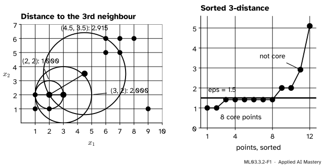
Each point’s distance to its third neighbour is the radius at which it becomes core when min_samples = 4. Sorted, the values form a flat run (points inside the squares) and then a steep rise (the edges and the strays). Every point at or below the line \(\varepsilon = 1.5\) is core.
Points inside a crowd collect their neighbours quickly, so their distances are small and similar: the flat part of the curve. Strays need a long way: the steep tail. A good \(\varepsilon\) sits where the curve turns from flat to steep, the knee. Below the knee most points are core; above it you would start to call strays core too.
Build it up
Step 1. One number per point. For a point \(\vect{x}\) write \(d_k(\vect{x})\) for its distance to its \(k\)-th nearest other point, its k-distance. With \(m = 4\) we use \(k = m - 1 = 3\). For \((2, 2)\), three other points lie at distance 1, so \(d_3 = 1\). For \((3, 2)\) the neighbours are at 1, 1.414 and 2, so \(d_3 = 2\).
Step 2. Sort. Put the twelve values in order: 1, 1, then six values of 1.414, then 2, 2, 2.915 and 5.099. That is the sorted k-distance plot of the anchor figure, the tool Ester et al. proposed in 1996. They plotted \(k = 4\) and set MinPts to 4 for two-dimensional data, which leaves a point at the threshold one neighbour to spare; \(k = m - 1\) is the exact count.
Step 3. Read off \(\varepsilon\). Choose \(\varepsilon\) at the knee, where the curve leaves its flat run. On the twelve points the flat run ends at 2 and the tail starts at 2.915, so any \(\varepsilon\) from about 1.5 to 2.9 gives the two groups; the worked example shows what changes inside that range.
Step 4. Choose \(m\) first. A larger \(m\) asks for denser crowds and smooths the k-distance curve; a smaller \(m\) lets tiny groups count as clusters. A common default is small and grows with the dimension: the original paper fixed 4 for points in the plane. Choose \(m\), then read \(\varepsilon\) from the plot for \(k = m - 1\).
Step 5. Standardise.\(\varepsilon\) is a distance, in the units of the data. If one feature is in metres and the other in kilometres, a circle of radius \(\varepsilon\) is a needle in one direction and a plate in the other. Scale the features first (ML01.3.3), then read the plot.
ML03.3.2-F2
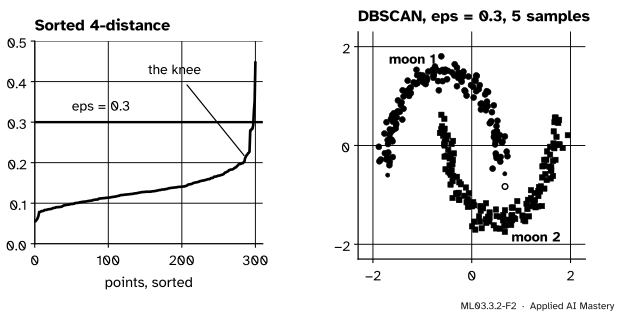
On 300 standardised points from make_moons, the sorted 4-distance plot bends sharply near 0.3. DBSCAN with that radius and min_samples = 5 finds both moons and calls one point noise; k-means, which cuts the plane in two straight halves, puts 48 points in the wrong moon.
The formal statement
NoteProposition: the k-distance decides the core points
Let \(m \ge 2\) and \(k = m - 1\). A point \(\vect{x}\) is a core point for \((\varepsilon, m)\) if and only if \(d_k(\vect{x}) \le \varepsilon\).
Proof. Order the other points by their distance to \(\vect{x}\), so that the \(j\)-th of them is at distance \(d_j(\vect{x})\), with \(d_1(\vect{x}) \le d_2(\vect{x}) \le \cdots\).
Suppose \(d_k(\vect{x}) \le \varepsilon\). Then the first \(k\) others are all within \(\varepsilon\). Together with \(\vect{x}\) itself, that is at least \(k + 1 = m\) points, so \(\vect{x}\) is core.
Suppose instead \(d_k(\vect{x}) > \varepsilon\). Then the \(k\)-th other point and every point after it lie outside the circle, so at most \(k - 1\) others are inside. With \(\vect{x}\) that is at most \(k = m - 1\) points, fewer than \(m\), so \(\vect{x}\) is not core. \(\square\)
Consequence 1: count the core points on the plot. The number of core points for a given \(\varepsilon\) is the number of values of the sorted plot at or below the line \(\varepsilon\).
Consequence 2: as \(\varepsilon\) grows, clusters of core points only merge. Fix \(m\) and take \(\varepsilon < \varepsilon'\). Every core point at \(\varepsilon\) is still core at \(\varepsilon'\), because \(d_k(\vect{x}) \le \varepsilon < \varepsilon'\). Two core points within \(\varepsilon\) of each other are still within \(\varepsilon'\). So every edge of the core graph at \(\varepsilon\) is still an edge at \(\varepsilon'\), and a connected piece stays connected. Each cluster’s core points at \(\varepsilon\) therefore lie inside a single cluster at \(\varepsilon'\): growing \(\varepsilon\) can merge clusters and add new points, but never split them.
Border points escape this rule. A border point can be within \(\varepsilon\) of two clusters, and then it goes to the one the search reaches first. That is the price of the definition, and the next two lessons build on Consequence 2 while treating border points with care.
Worked example
The twelve points with min_samples = 4, for every \(\varepsilon\). The 3-distances are 1.414 for \((1, 1)\), \((2, 1)\), \((1, 2)\) and the same three corners of the upper square, 1 for \((2, 2)\) and \((7, 6)\), 2 for \((3, 2)\) and \((8, 6)\), then \(\sqrt{8.5} \approx 2.915\) for the bridge and \(\sqrt{26} \approx 5.099\) for \((9, 1)\). By the proposition, each value is the radius at which its point becomes core. Raise \(\varepsilon\) and points switch on one value at a time:
\(\varepsilon\) from
new core points
clusters
1
\((2, 2)\), \((7, 6)\)
two of four
1.414
six more corners
two of five
2
\((3, 2)\), \((8, 6)\)
two of five
2.915
the bridge
one of eleven
5.099
\((9, 1)\)
one of twelve
Below 1 there is no core point and all twelve are noise. Between 1 and 1.414 only \((2, 2)\) and \((7, 6)\) are core; their circles of radius at least 1 take in the three points at distance 1, so each cluster has four, and \((1, 1)\) and \((6, 5)\) are noise.
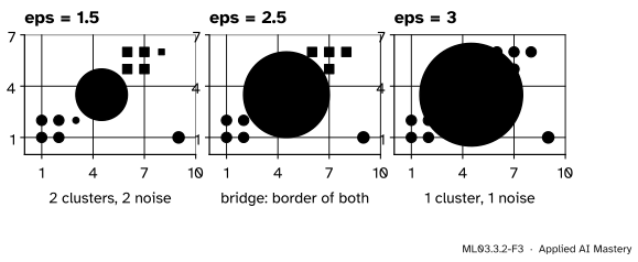
Two events happen between the rows. At \(\varepsilon = \sqrt{4.5} \approx 2.121\) the bridge comes within reach of the core points \((3, 2)\) and \((6, 5)\), but it is not core itself (its 3-distance is 2.915): it becomes a border point of both clusters. At \(\varepsilon = \sqrt{20} \approx 4.472\), \((9, 1)\) comes within reach of the core point \((7, 5)\) and joins as a border point, before it becomes core at 5.099.
ML03.3.2-F3
Three frames of the same data. At \(\varepsilon = 2.5\) the bridge is a border point of both groups and joins the one found first. At \(\varepsilon = 3\) it is core, and the chain through it merges the groups.
So the knee, between 2 and 2.915, is a range, not a number. Anywhere in it the two groups are found, but above 2.121 the bridge is handed to one of them on a technicality. The cautious choice is the bottom of the range, \(\varepsilon = 2\), or a little below it: 1.5 gives the same two groups.
Code
NearestNeighbors finds each point’s neighbours with a tree. Asked about the training points themselves, it returns each point as its own nearest neighbour, at distance 0, so the last of min_samples columns is exactly \(d_{m-1}\).
Now the moons, standardised first. The tail of the sorted 4-distance plot rises sharply near 0.3.
Xm, ym = make_moons(n_samples=300, noise=0.07, random_state=0)Z = StandardScaler().fit_transform(Xm)kd_m = np.sort(kdistance(Z, 5))print("median and last five 4-distances:", round(np.median(kd_m), 3), np.round(kd_m[-5:], 3))db = DBSCAN(eps=0.3, min_samples=5).fit(Z)km = KMeans(n_clusters=2, n_init=10, random_state=0).fit(Z)same =lambda labels: max((labels == ym).sum(), (labels ==1- ym).sum()) # either numberingprint("DBSCAN clusters:", db.labels_.max() +1, " noise:", (db.labels_ ==-1).sum()," in the right moon:", same(db.labels_))print("k-means points in the right moon:", same(km.labels_))Xu = Xm * [1, 1000] # the second feature in different unitsprint("unscaled, eps = 0.3: noise", (DBSCAN(eps=0.3, min_samples=5).fit(Xu).labels_ ==-1).sum())
median and last five 4-distances: 0.128 [0.283 0.292 0.327 0.352 0.448]
DBSCAN clusters: 2  noise: 1  in the right moon: 299
k-means points in the right moon: 252
unscaled, eps = 0.3: noise 300
DBSCAN puts 299 of the 300 points in the right moon; k-means gets 252, 48 wrong. With the second feature in units a thousand times smaller, no point has a neighbour within 0.3 and all 300 are noise.
The failures. First, blobs of two densities: two tight blobs 1.2 apart and one wide blob. Scan \(\varepsilon\) and ask whether any value gives each blob its own cluster.
from sklearn.datasets import make_blobsXb, yb = make_blobs(n_samples=[100, 100, 100], centers=[(0, 0), (1.2, 0), (4.5, 3)], cluster_std=[0.15, 0.15, 1.5], random_state=1)def recovers_blobs(labels, y):"""True when three different clusters each hold at least 70 of one blob's 100 points.""" tops = []for g inrange(3): counts = np.bincount(labels[(y == g) & (labels >=0)], minlength=1) tops.append((counts.argmax(), counts.max()))returnlen({k for k, _ in tops}) ==3andmin(c for _, c in tops) >=70grid = np.round(np.arange(0.02, 2.0001, 0.01), 2)found = [e for e in grid if recovers_blobs(DBSCAN(eps=e, min_samples=5).fit(Xb).labels_, yb)]for e in (0.2, 0.7): lab = DBSCAN(eps=e, min_samples=5).fit(Xb).labels_print(f"eps {e}: clusters {lab.max() +1}, noise {(lab ==-1).sum()}")print("values of eps that recover the three blobs:", found)
eps 0.2: clusters 2, noise 98
eps 0.7: clusters 2, noise 19
values of eps that recover the three blobs: []
Second, many dimensions. For 500 uniform points, compare the largest and smallest 4-distance.
ratios = {}for d in (2, 100): A = np.random.default_rng(0).uniform(size=(500, d)) kd_d = kdistance(A, 5) ratios[d] = kd_d.max() / kd_d.min()print(f"d = {d}: largest / smallest 4-distance = {ratios[d]:.2f}")
d = 2: largest / smallest 4-distance = 7.63
d = 100: largest / smallest 4-distance = 1.17
In the plane the loneliest point needs a radius 7.6 times the busiest one’s. In 100 dimensions the two differ by 17 percent: there is no knee to find.
Explore
ML03.3-X1
DBSCAN explorer
Slide eps and step min_samples on the twelve points: every point is redrawn as core, border or noise, and the sorted k-distance plot beneath moves its line with you. Press Grow one step to watch a cluster spread one point at a time, and tap the plane (or press Add point) to add up to twenty points of your own. Try eps = 2.5 and look at the bridge.
Pitfalls
ML03.3.2-F4
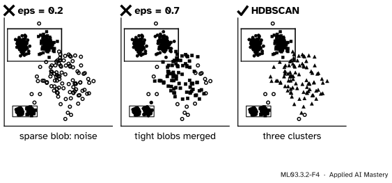
Wrong beside right. A radius small enough to keep the tight blobs apart dissolves the sparse blob into noise; a radius large enough for the sparse blob merges the tight ones. HDBSCAN (ML03.3.4) finds all three.
“There is always a right eps; I just have to find it.”
One \(\varepsilon\) means one density threshold for the whole data set. When clusters differ in density, no value serves them all: on the blobs above, no \(\varepsilon\) from 0.02 to 2 gives each blob its own cluster holding at least 70 of its 100 points. The remedy is to stop choosing one \(\varepsilon\): OPTICS (next lesson) looks at all of them, and HDBSCAN picks clusters at different densities.
ML03.3.2-F5
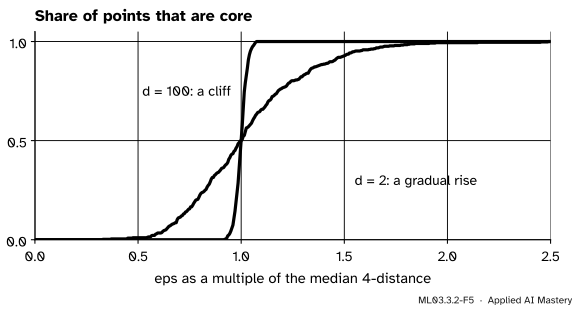
In two dimensions the share of core points rises gradually as \(\varepsilon\) grows. In 100 dimensions every point’s 4-distance is nearly the same, so the share jumps from none to all.
“DBSCAN works the same in any number of dimensions.”
In high dimensions distances concentrate (ML01.3.4): the nearest and the farthest neighbours are almost equally far. The k-distance plot loses its knee, and \(\varepsilon\) switches from “everything is noise” to “everything is core” within a few percent. Reduce the dimension first (PCA, ML03.5), or use a distance that suits the data.
ML03.3.2-F6
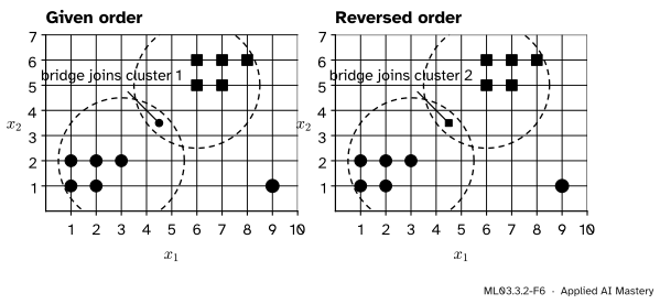
At \(\varepsilon = 2.5\) the bridge is a border point of both clusters. Run on the data as given, it joins cluster 1; run on the same points in reverse order, it joins cluster 2.
“DBSCAN’s answer does not depend on the order of the rows.”
The core points and the clusters of core points do not. A border point within reach of two clusters goes to the first cluster that reaches it, so shuffling the rows can move it, as the figure shows. The scikit-learn guide says so: such a sample “is assigned to whichever cluster is generated first”. If border points matter, report them, or use a method without them (HDBSCAN’s DBSCAN*, ML03.3.4).
Check yourself
Recall
1. With min_samples = m, which neighbour’s distance decides whether a point is core?
Show answer
Its distance to its \((m - 1)\)-th nearest other point: the point is core exactly when that distance is at most \(\varepsilon\).
2. On a sorted k-distance plot, which part is the clusters and which part is the noise?
Show answer
The long flat run of small values is the points inside clusters; the steep tail of large values is the sparse points and strays.
3. Why must features be standardised before choosing \(\varepsilon\)?
Show answer
\(\varepsilon\) is a distance in the units of the data. A feature measured in large units dominates the distance, so the circle is squashed in the other directions.
4. As \(\varepsilon\) grows with \(m\) fixed, can two core points in the same cluster end up in different clusters?
Show answer
No. Core points stay core and edges of the core graph stay edges, so clusters of core points can only merge.
5. Name the three situations where DBSCAN fails.
Show answer
Clusters of different density (no single \(\varepsilon\) serves them), high-dimensional data (distances concentrate and the knee disappears), and border points within reach of two clusters (the result depends on the order of the data).
Exercises
1.★ The sorted 3-distances of a data set are 0.2, 0.2, 0.3, 0.3, 0.3, 0.4, 0.4, 0.5, 1.8 and 2.6. With min_samples = 4, how many points are core for \(\varepsilon = 0.35\) and for \(\varepsilon = 0.5\), and where would you put \(\varepsilon\)?
Show solution
By the proposition, a point is core when its 3-distance is at most \(\varepsilon\).
For \(\varepsilon = 0.35\): the values 0.2, 0.2, 0.3, 0.3, 0.3 qualify, so 5 points are core.
For \(\varepsilon = 0.5\): the eight values up to 0.5 qualify, so 8 points are core.
The curve is flat up to 0.5 and then jumps to 1.8: the knee lies between them. Any \(\varepsilon\) from 0.5 to just under 1.8 makes the eight crowded points core and leaves the last two out; the cautious choice is near 0.5.
2.★★ Using the table of the worked example, give the clusters, border points and noise of the twelve points for min_samples = 4 and \(\varepsilon = 1.2\).
Show solution
At \(\varepsilon = 1.2\) the core points are those with a 3-distance of at most 1.2: only \((2, 2)\) and \((7, 6)\), with 3-distance 1.
The circle of \((2, 2)\) contains the points at distance at most 1.2: \((2, 1)\), \((1, 2)\) and \((3, 2)\), all at distance 1. They are not core, so the chain stops: cluster 1 is \((2, 2)\) with the border points \((2, 1)\), \((1, 2)\), \((3, 2)\). In the same way cluster 2 is \((7, 6)\) with the border points \((7, 5)\), \((6, 6)\) and \((8, 6)\).
The corners \((1, 1)\) and \((6, 5)\) are \(\sqrt{2} \approx 1.414 > 1.2\) from the core points, so they are noise, together with the bridge and \((9, 1)\): four noise points in all.
3.★★★ Show that if \(\varepsilon \le \varepsilon'\) and \(m' \le m\), every core point for \((\varepsilon, m)\) is a core point for \((\varepsilon', m')\), and deduce how lowering min_samples changes the clusters of core points.
Show solution
If \(\vect{x}\) is core for \((\varepsilon, m)\), then \(\abs{N_\varepsilon(\vect{x})} \ge m\). Every point within \(\varepsilon\) is also within \(\varepsilon'\), so the neighbourhood can only grow:
\[
\abs{N_{\varepsilon'}(\vect{x})} \ge \abs{N_\varepsilon(\vect{x})} \ge m \ge m'.
\]
So \(\vect{x}\) is core for \((\varepsilon', m')\).
Now keep \(\varepsilon\) fixed and lower \(m\) to \(m'\). Every old core point is still core, and the edges between core points depend only on \(\varepsilon\), so every old edge remains. As in Consequence 2, each old cluster’s core points stay connected and lie inside one new cluster. Lowering min_samples can only add core points and merge clusters, never split them.
Summary card
Sort each point’s distance to its (m - 1)-th neighbour, and put eps at the knee.
ML03.3.2-F1
The sorted k-distance plot.
Core test.\(\vect{x}\) is core for \((\varepsilon, m)\) exactly when \(d_{m-1}(\vect{x}) \le \varepsilon\).
Choosing. Fix \(m\), standardise, plot the sorted \(d_{m-1}\), put \(\varepsilon\) at the knee.
Nesting. Growing \(\varepsilon\) or shrinking \(m\) only merges clusters of core points.
Failures. Mixed densities, many dimensions, and border points claimed by two clusters.
Sources and next steps
Sources. Each was opened and checked against this lesson on 15 November 2026.
Martin Ester, Hans-Peter Kriegel, Jörg Sander and Xiaowei Xu, A density-based algorithm for discovering clusters in large spatial databases with noise, KDD-96. Section 4.2 introduces the sorted k-dist graph, reads the threshold at the first “valley”, and fixes MinPts at 4 for two-dimensional data; section 4.1 notes that a point that is a border point of two clusters is assigned to the cluster discovered first.
scikit-learn developers, User Guide, section 2.3.7 DBSCAN, version 1.9: a non-core sample “is assigned to whichever cluster is generated first in a pass through the data, and so the results will depend on the data ordering”.