Internal indices: the silhouette and its relatives
With no labels, a clustering can only be judged by how tight and how separated its clusters are. Compute the silhouette of every point, read a silhouette plot, define the Calinski-Harabasz and Davies-Bouldin indices, and see why all of them favour round clusters.
ML03.10.1L2 Intermediate25 minIn review (what this means)
The maths and code on this page are checked by automated tests on every change, but an independent reader has not signed it off yet. Spot a mistake or a confusing step? Tell us.
Compute the silhouette of a point from its mean distance to its own cluster and to the nearest other cluster, and read a silhouette plot.
Use the mean silhouette to compare clusterings and to choose the number of clusters K.
Define the Calinski-Harabasz and Davies-Bouldin indices and compute both from scratch and with scikit-learn.
Explain why every internal index favours compact, round clusters, and show a case where it prefers the wrong answer.
The question
k-means hands you two clusters of the nine points. There are no labels to check them against, and its own score \(J\) always improves when you ask for more clusters. So how good is this clustering, which point is badly placed, and is two the right number of clusters at all?
Intuition
A good clustering has two properties. Each point is close to its own cluster and far from the others. The silhouette turns both into one number per point, by comparing two average distances.
ML03.10.1-F1
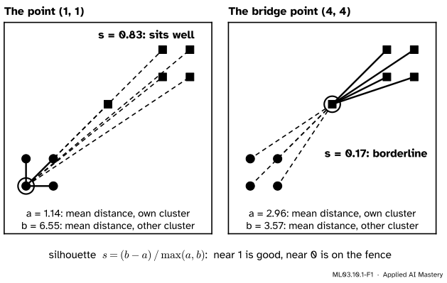
The silhouette of a point compares \(a\), its mean distance to its own cluster, with \(b\), its mean distance to the nearest other cluster. The corner point \({(1, 1)}\) has \(b\) far larger than \(a\) and scores \(0.83\). The bridge point \({(4, 4)}\) is almost as close to the other cluster as to its own, and scores only \(0.17\).
Read the two panels. For \({(1, 1)}\) the solid lines are short and the dashed lines long: the point clearly belongs where it is. For the bridge point the two kinds of line are of similar length: it sits on the fence. A point whose dashed lines were shorter than its solid lines would be in the wrong cluster, and its silhouette would be negative.
Average the silhouettes of all the points and you have a score for the whole clustering, one that does not simply improve as \(K\) grows, unlike \(J\).
Build it up
Step 1. Tightness. For point \(i\) in cluster \(C\), let \({a(i)}\) be the mean distance from \(i\) to the other points of \(C\). Small \({a(i)}\) means a tight cluster around \(i\).
Step 2. Separation. For every other cluster, take the mean distance from \(i\) to its points. The smallest of these is \({b(i)}\): the distance to the nearest other cluster, the one \(i\) would join if its own cluster vanished.
Step 3. One number. The silhouette of \(i\) is the gap between the two, scaled by the larger: \({s(i)} = {(b - a)/\max(a, b)}\). Dividing makes it free of units, so it lies between \(-1\) and \(1\).
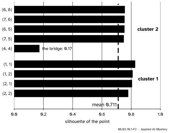
Step 4. The silhouette plot. Draw one horizontal bar per point, of length \({s(i)}\), sorted within each cluster. Thin or negative bars show at a glance which points are badly placed and which clusters are loose.
ML03.10.1-F2
The silhouette plot of the nine points with \({K} = {2}\). Eight bars are long; the bridge point’s is short. Their mean, \(0.711\), scores the whole clustering.
Step 5. Choosing K. Compute the mean silhouette for each candidate \(K\) and prefer the largest. On the nine points, \({K} = {2}\) gives \(0.711\). With \({K} = {3}\) the best clustering puts the bridge point in a cluster of its own; a point alone gets \({s} = {0}\) by convention, and the mean falls to \(0.568\). So the silhouette prefers two clusters.
The formal statement
NoteDefinition: silhouette
Let \(d_{ij}\) be the distance between points \(i\) and \(j\), and let point \(i\) lie in cluster \(C_i\) with at least one other point. Then
A point alone in its cluster gets \({s(i)} = {0}\). The mean silhouette is the average of \({s(i)}\) over all \(n\) points. It needs \({2 \le K \le n - 1}\).
Why \(s\) lies between \(-1\) and \(1\). If \({a < b}\), the maximum is \(b\) and \({s} = {1 - a/b}\); since \({0} \le {a/b < 1}\), \(s\) lies in \({(0, 1]}\). If \({a > b}\), the maximum is \(a\) and \({s} = {b/a - 1}\); since \({0} \le {b/a < 1}\), \(s\) lies in \({[-1, 0)}\). If \({a} = {b}\), \({s} = {0}\). So \(s\) near \(1\) means \(a\) is tiny next to \(b\), and \(s\) near \(-1\) means the point is far closer to another cluster.
Two more indices score a whole clustering from its centres. Write \(\vect{\mu}_k\) for the mean of cluster \(k\), \(n_k\) for its size and \(\bar{\vect{x}}\) for the mean of all the data.
Calinski-Harabasz. Split the scatter of the data about \(\bar{\vect{x}}\) into a part within the clusters, \(W\), which is exactly the \(J\) of k-means, and a part between them, \(B\):
Large \(B\) and small \(W\) give a large CH. The divisors \({K - 1}\) and \({n - K}\) stop CH from rising just because \(K\) grows, as in an analysis of variance.
Go deeper: the total scatter splits exactly into B plus W
For a point \(\vect{x}_i\) in cluster \(k\), write \({\vect{x}_i - \bar{\vect{x}}} = {(\vect{x}_i - \vect{\mu}_k)} + {(\vect{\mu}_k - \bar{\vect{x}})}\). Square the length and expand:
Sum over the points of cluster \(k\). The first terms add to that cluster’s share of \(W\). The second term does not depend on \(i\), so it adds to \({n_k \norm{\vect{\mu}_k - \bar{\vect{x}}}^2}\). In the cross term, \({\sum_{i \in C_k} (\vect{x}_i - \vect{\mu}_k)} = {\vect{0}}\), because \(\vect{\mu}_k\) is the mean of those points, so it vanishes. Summing over \(k\) gives total scatter \(= {W} + {B}\).
Davies-Bouldin. Let \(s_k\) be the mean distance from the points of cluster \(k\) to \(\vect{\mu}_k\) (its spread), and \({d_{kl}} = {\norm{\vect{\mu}_k - \vect{\mu}_l}}\). For each cluster, find its worst neighbour and average:
Small is good: spreads small next to the distances between centres. Zero is the best possible.
ML03.10.1-F3
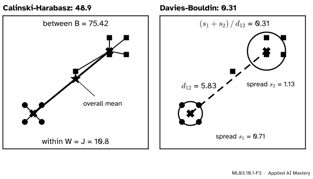
What the two centre-based indices measure. Left: Calinski-Harabasz compares the scatter of the centres about the overall mean (\(B\)) with the scatter of the points about their centres (\(W\)). Right: Davies-Bouldin compares each cluster’s spread with the distance between centres.
Worked example
The bridge point \({(4, 4)}\), with the lower square and the upper five as clusters.
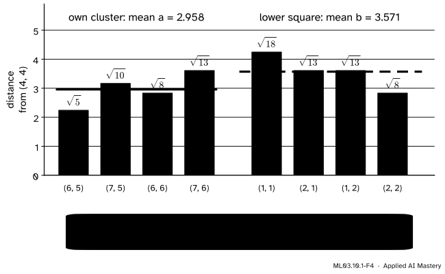
Its own cluster. The other four upper points are \({(6, 5)}\), \({(7, 5)}\), \({(6, 6)}\) and \({(7, 6)}\), at distances \({\sqrt{5}}\), \({\sqrt{10}}\), \({\sqrt{8}}\) and \({\sqrt{13}}\). Their mean is
The silhouette. Here \({b > a}\), so the maximum is \(b\) and \({s} = {(3.571 - 2.958)/3.571} = {0.172}\).
ML03.10.1-F4
The bridge point’s silhouette, step by step: eight distances, two means, one ratio. The means \(2.958\) and \(3.571\) are close, so \(s\) is small.
The other eight points are worked the same way; \({(1, 1)}\), for example, has \({a} = {(1 + 1 + \sqrt{2})/3} = {1.138}\) and \({b} = {6.548}\), so \({s} = {1 - 1.138/6.548} = {0.826}\). The nine silhouettes average to \(0.711\).
The two centre-based indices. The centres are \({(1.5, 1.5)}\) and \({(6, 5.2)}\), and the overall mean is \({(4, 32/9)} \approx {(4, 3.556)}\). Then \({W} = {J} = {10.8}\) and
So \({\mathrm{CH}} = {(75.42/1)\,/\,(10.8/7)} = {48.88}\). For Davies-Bouldin, every lower point is \({\sqrt{0.5}} = {0.707}\) from its centre, so \({s_1} = {0.707}\); the upper five are \(0.2\), \(1.020\), \(0.8\), \(1.281\) and \(2.332\) from theirs, so \({s_2} = {1.127}\). The centres are \({d_{12}} = {\sqrt{4.5^2 + 3.7^2}} = {5.826}\) apart, and with two clusters both have the same worst neighbour, so \({\mathrm{DB}} = {(0.707 + 1.127)/5.826} = {0.315}\).
Code
The three indices from scratch, checked against scikit-learn on the nine points.
import numpy as npfrom sklearn.metrics import (calinski_harabasz_score, davies_bouldin_score, silhouette_samples, silhouette_score)def silhouettes(X, z): D = np.sqrt(((X[:, None, :] - X[None, :, :]) **2).sum(-1)) s = np.zeros(len(X))for i inrange(len(X)): own = (z == z[i]) & (np.arange(len(X)) != i)ifnot own.any():continue# alone in its cluster: s = 0 a = D[i, own].mean() b =min(D[i, z == k].mean() for k in np.unique(z) if k != z[i]) s[i] = (b - a) /max(a, b)return sdef calinski_harabasz(X, z): ks = np.unique(z); centre = X.mean(0) W =sum(((X[z == k] - X[z == k].mean(0)) **2).sum() for k in ks) B =sum((z == k).sum() * ((X[z == k].mean(0) - centre) **2).sum() for k in ks)return (B / (len(ks) -1)) / (W / (len(X) -len(ks))), B, Wdef davies_bouldin(X, z): ks = np.unique(z); mu = np.array([X[z == k].mean(0) for k in ks]) s = np.array([np.linalg.norm(X[z == k] - mu[i], axis=1).mean() for i, k inenumerate(ks)]) R = [max((s[i] + s[j]) / np.linalg.norm(mu[i] - mu[j]) for j inrange(len(ks)) if j != i)for i inrange(len(ks))]return np.mean(R)X = np.array([(1, 1), (2, 1), (1, 2), (2, 2), (6, 5), (7, 5), (6, 6), (7, 6), (4, 4)], float)z = np.array([0, 0, 0, 0, 1, 1, 1, 1, 1])s = silhouettes(X, z)ch, B, W = calinski_harabasz(X, z)print("silhouettes:", s.round(3), " mean:", round(s.mean(), 3))print(f"B = {B:.2f}, W = {W:.1f}, CH = {ch:.2f}, DB = {davies_bouldin(X, z):.3f}")
silhouettes: [0.826 0.805 0.809 0.779 0.753 0.749 0.756 0.754 0.172]  mean: 0.711
B = 75.42, W = 10.8, CH = 48.88, DB = 0.315
Now the bridge point alone, as \({K} = {3}\): the indices disagree. The silhouette prefers \({K} = {2}\), while CH and DB prefer \({K} = {3}\), because a cluster of one point has no spread at all.
K = 2: silhouette 0.512   CH   363.6   DB 0.802
K = 3: silhouette 0.529   CH   317.5   DB 0.773
K = 4: silhouette 0.617   CH   463.2   DB 0.607
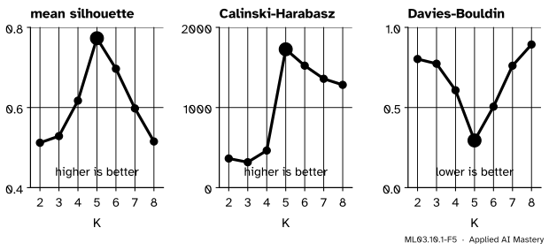
K = 5: silhouette 0.773   CH  1726.5   DB 0.294
K = 6: silhouette 0.697   CH  1522.2   DB 0.506
K = 7: silhouette 0.598   CH  1358.3   DB 0.761
K = 8: silhouette 0.515   CH  1282.7   DB 0.893
ML03.10.1-F5
On well-separated round blobs all three indices agree: the best \(K\) is \(5\).
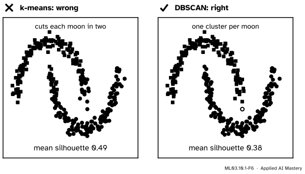
Last, the moons of ML03.3.2, where DBSCAN found both moons and k-means cut them straight across.
from sklearn.cluster import DBSCANfrom sklearn.datasets import make_moonsfrom sklearn.preprocessing import StandardScalerXm, _ = make_moons(n_samples=300, noise=0.07, random_state=0)Zm = StandardScaler().fit_transform(Xm)db = DBSCAN(eps=0.3, min_samples=5).fit_predict(Zm)km = KMeans(2, n_init=10, random_state=0).fit_predict(Zm)keep = db !=-1# leave out DBSCAN's one noise pointfor name, M, lab in [("k-means", Zm, km), ("DBSCAN", Zm[keep], db[keep])]:print(f"{name:8s} silhouette {silhouette_score(M, lab):.3f} CH {calinski_harabasz_score(M, lab):6.1f}"f" DB {davies_bouldin_score(M, lab):.3f}")
k-means  silhouette 0.492   CH  412.7   DB 0.810
DBSCAN   silhouette 0.383   CH  255.7   DB 1.026
All three indices prefer k-means’ wrong answer: silhouette \(0.49\) against \(0.38\), CH \(412.7\) against \(255.7\), DB \(0.81\) against \(1.03\).
Explore
The cluster scorecard, in lesson ML03.10.3, shows every point’s silhouette as a bar and the mean silhouette and Davies-Bouldin index in its read-out. Choose moons and slide \(K\): the best silhouette never belongs to the two true moons.
Pitfalls
ML03.10.1-F6
Wrong beside right. k-means cuts each moon in two yet scores the higher mean silhouette, \(0.49\); DBSCAN’s correct moons score \(0.38\), because the ends of each moon are far from its middle.
“The clustering with the higher silhouette is the right one.”
Only if the right clusters are compact and round. The silhouette, CH and DB all reward small distances within a cluster, so an elongated or curved cluster is penalised however real it is. The scikit-learn user guide warns of exactly this for density-based clusters such as DBSCAN’s. Judge non-convex clusters by looking, by stability (ML03.10.3) or by known labels (ML03.10.2).
“The indices agree, so I can use any of them.”
On the nine points the silhouette picks \({K} = {2}\), and CH and DB pick \({K} = {3}\), with the bridge point alone. Each index encodes a different idea of a good cluster. Report more than one, and look.
“A mean silhouette of 0.5 means there are clusters.”
Uniform noise, with no clusters at all, clustered by k-means with \({K} = {2}\) scores \(0.48\) in ML03.10.3. An internal index measures how good the partition is, not whether the data have groups. The scores also depend on the scale of each feature, so standardise first (ML01.3.3) and never compare silhouettes across different data sets.
Check yourself
Recall
1. What are \({a(i)}\) and \({b(i)}\) in the silhouette of point \(i\)?
Show answer
\({a(i)}\) is the mean distance from \(i\) to the other points of its own cluster; \({b(i)}\) is the smallest mean distance from \(i\) to the points of another cluster.
2. What does a negative silhouette tell you?
Show answer
That \({a > b}\): the point is closer, on average, to another cluster than to its own, so it is probably in the wrong cluster.
3. What silhouette does a point alone in its cluster get, and why does it matter for choosing \(K\)?
Show answer
\(0\), by convention. Splitting points off into clusters of one therefore lowers the mean silhouette, which keeps it from rewarding ever larger \(K\).
4. In the Calinski-Harabasz index, what are \(B\) and \(W\), and what is \({B} + {W}\)?
Show answer
\(W\) is the within-cluster sum of squares (the \(J\) of k-means), \(B\) the size-weighted scatter of the centres about the overall mean, and \({B} + {W}\) is the total scatter about the overall mean.
5. Is a large or a small Davies-Bouldin index better, and what does it compare?
Show answer
Small. For each cluster it takes the worst ratio of the two clusters’ spreads to the distance between their centres, and averages over clusters.
Exercises
1.★ A point has mean distance \(2\) to its own cluster and mean distances \(5\) and \(3\) to two other clusters. Find its silhouette.
Show solution
\({a} = {2}\), and \(b\) is the smaller of the other means, \(3\). Since \({b > a}\), \({s} = {(3 - 2)/3} = {0.333}\). The cluster at distance \(5\) plays no part.
2.★★ Put the bridge point in the lower group instead. Find its new silhouette and explain the sign.
Show solution
Now its own cluster is the lower square, at mean distance \(3.571\), and the nearest other cluster is the four upper points, at mean distance \(2.958\). So \({a} = {3.571}\), \({b} = {2.958}\), and since \({a > b}\), \({s} = {(2.958 - 3.571)/3.571} = {-0.172}\). The two means simply swap, so the silhouette changes sign. It is negative because the point is now in the cluster that is farther away. The mean over all nine points falls to \(0.661\).
3.★★★ Show that \({\mathrm{CH}} = {\dfrac{(T - W)/(K - 1)}{W/(n - K)}}\), where \(T\) is the total scatter, and use it to explain why, for fixed \(K\), the clustering with the highest CH is the one with the lowest \(J\).
Show solution
The deeper block shows that \({T} = {B} + {W}\), so \({B} = {T - W}\). Substitute into the definition of CH. For fixed data \(T\), \(n\) and \(K\) do not depend on the clustering, so CH is a function of \(W\) alone. Write \({c} = {(n - K)/(K - 1) > 0}\); then \({\mathrm{CH}} = {c\,(T - W)/W} = {c\,(T/W - 1)}\), which falls as \(W\) grows. So among clusterings with the same \(K\), the highest CH has the smallest \(W\), which is the \(J\) of k-means. CH only adds something when it compares different values of \(K\).
Summary card
A clustering without labels is judged by how tight and how separated its clusters are.
ML03.10.1-F1
Own cluster against the nearest other.
Silhouette.\({s} = {(b - a)/\max(a, b)}\), from \(-1\) to \(1\); average it over the points.
Calinski-Harabasz.\({\mathrm{CH}} = {\dfrac{B/(K - 1)}{W/(n - K)}}\), larger is better.
Davies-Bouldin. Mean over clusters of \({\max_l (s_k + s_l)/d_{kl}}\), smaller is better.
Nine points. Mean silhouette \(0.711\), bridge \(0.172\); CH \(48.88\); DB \(0.315\).
Limit. All three favour round, compact clusters, and none tests whether any exist.
Sources and next steps
Sources. Each was opened and checked against this lesson on 15 November 2026.
scikit-learn developers, User Guide, Section 2.3.11 Clustering performance evaluation, version 1.9. Section 2.3.11.5 defines the silhouette as \({(b - a)/\max(a, b)}\) with \(a\) the mean distance to the same class and \(b\) to the next nearest cluster; 2.3.11.6 gives Calinski-Harabasz as the ratio of the traces of \(B_k\) and \(W_k\) times \({(n_E - k)/(k - 1)}\); 2.3.11.7 gives Davies-Bouldin with \({R_{ij}} = {(s_i + s_j)/d_{ij}}\). Each of the three sections warns that its index favours convex clusters over density-based clusters such as DBSCAN’s.
scikit-learn developers, sklearn.metrics.silhouette_samples, version 1.9. The silhouette is defined only for \({2} \le\) number of labels \(\le {n - 1}\), ranges from \(-1\) to \(1\), and is credited to Rousseeuw (1987), Journal of Computational and Applied Mathematics 20, 53 to 65. That the library scores a point alone in its cluster as \(0\) is checked in the code above.
Trevor Hastie, Robert Tibshirani and Jerome Friedman, The Elements of Statistical Learning, 2nd edition. Section 14.3.11 explains why the within-cluster scatter \(W_K\) falls as \(K\) grows, so that it cannot choose \(K\) by itself.