Is there any structure? Stability and the gap statistic
Every clustering algorithm returns clusters, even from uniform noise. Compare log W with its value on uniform reference data (the gap statistic), check whether the clusters survive resampling (stability), and learn where each test, and BIC, can still be fooled.
ML03.10.3L2 Intermediate25 minIn review (what this means)
The maths and code on this page are checked by automated tests on every change, but an independent reader has not signed it off yet. Spot a mistake or a confusing step? Tell us.
Show that k-means and the silhouette report clusters in uniform noise, and explain why an internal index cannot detect that.
Compute the gap statistic with uniform reference data and choose K by the one-standard-error rule.
Measure the stability of a clustering by comparing fits on overlapping subsamples with the adjusted Rand index.
State the limits of the gap statistic, of stability and of BIC, and give a data set that fools each.
The question
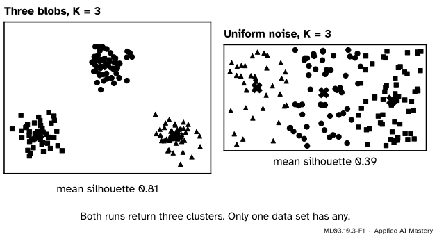
Run k-means with \({K} = {3}\) on points scattered uniformly in a rectangle. It returns three neat clusters, and their mean silhouette is \(0.39\). Nothing told you that the data had no clusters to find. How can you test whether a clustering has found structure, or merely carved up noise?
From the last lesson
1. What is the adjusted Rand index of the six points, truth \({(a, a, a, b, b, b)}\) against clusters \({(1, 1, 2, 2, 3, 3)}\)?
Its chance level is well above 0 and depends on the number of clusters: random labels of iris score about \(0.56\) with 3 clusters and \(0.64\) with 10.
Intuition
An algorithm answers the question you asked. Ask k-means for three clusters and it returns three, whatever the data look like. An internal index such as the silhouette then scores the partition, and a uniform cloud cut into three pieces is a perfectly respectable partition.
ML03.10.3-F1
The same algorithm with the same \(K\) on two data sets. Only the left one has clusters, yet both runs return three, and the noise still earns a mean silhouette of \(0.39\).
Two ideas test for structure. The first asks how much better than noise the clustering is: cluster data that are known to have no groups, spread over the same region, and compare. That is the gap statistic. The second asks whether the answer is reproducible: cluster two random halves of the data and check that they agree. That is stability.
Build it up
Step 1. Within-cluster scatter always falls. Let \(W_K\) be the \(J\) of the best \(K\)-means clustering. It falls as \(K\) grows on any data (ML03.1.3), so its size alone says nothing.
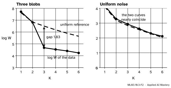
Step 2. Compare with noise. Draw uniform points in the bounding box of the data, the smallest box with sides parallel to the axes that holds every point, and cluster them too. Their \(W_K\) also falls, but at the rate noise falls. Work with \({\log W_K}\), so that only the rate matters, not the overall scale.
ML03.10.3-F2
\({\log W_K}\) for the data (solid) and its average over 20 uniform reference data sets (dashed). For the blobs the data curve plunges below the reference at \({K} = {3}\); for noise the two curves run together.
Step 3. The gap. The gap at \(K\) is the reference curve minus the data curve. A big gap means the data cluster far better than noise with that \(K\). Choose the smallest \(K\) whose gap is not clearly beaten by \({K} + {1}\).
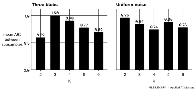
Step 4. Stability. Draw two random subsamples of 80 percent of the points, cluster each with the same \(K\), and compare the two labellings on the points they share by the adjusted Rand index of ML03.10.2. Repeat and average. A real \(K\) gives the same answer every time; a wrong one cuts a group in different places each time.
ML03.10.3-F4
Stability for \({K} = {2}\) to \(6\). For the blobs it peaks at \(1.00\) at \({K} = {3}\). For the noise it is highest at \({K} = {2}\), \(0.96\): a stable answer to a question with no answer.
The formal statement
NoteThe gap statistic (Tibshirani, Walther and Hastie, 2001)
Step 1. Cluster the data for \({K = 1, \dots, K_{\max}}\) and record \(W_K\), the pooled within-cluster sum of squares.
Step 2. Draw \(B\) reference data sets, each uniform over the range of every feature, cluster each for every \(K\), and record \(W^*_{Kb}\). Then
where \(\mathrm{sd}_K\) is the standard deviation of the \(B\) values \({\log W^*_{Kb}}\).
Step 3. Choose the smallest \(K\) with \({\mathrm{Gap}(K)} \ge {\mathrm{Gap}(K + 1) - s_{K+1}}\).
The factor \({\sqrt{1 + 1/B}}\) adds the error of estimating the reference mean from only \(B\) samples. The rule is a one-standard-error rule: move to \({K} + {1}\) only when it is clearly better. Because \({K} = {1}\) is allowed, the gap can answer “no clusters”, which the silhouette, needing \({K \ge 2}\), cannot.
Go deeper: W from pairwise distances, as the paper defines it
Tibshirani and colleagues write \({W_K} = {\sum_r D_r / (2 n_r)}\), where \(D_r\) sums the squared distances over all ordered pairs of points in cluster \(r\). This is the within-cluster sum of squares. For one cluster with mean \(\vect{\mu}\), write \({\vect{x}_i - \vect{x}_j}\) as \({(\vect{x}_i - \vect{\mu}) - (\vect{x}_j - \vect{\mu})}\) and expand:
Each of the first two sums is \(n\) times \({\sum_i \norm{\vect{x}_i - \vect{\mu}}^2}\), and the last term is zero because \({\sum_i (\vect{x}_i - \vect{\mu})} = {\vect{0}}\). So \({D} = {2n \sum_i \norm{\vect{x}_i - \vect{\mu}}^2}\), and \({D/(2n)}\) is that cluster’s share of \(J\).
Stability. For each \(K\), repeat \(m\) times: draw two subsamples without replacement, cluster each, and compute the ARI of the two labellings on the shared points. The stability of \(K\) is the mean ARI; prefer the \(K\) where it is high. von Luxburg’s survey lists this protocol (overlapping subsamples, Ben-Hur and colleagues 2002) among several that differ in how the data are perturbed and how labellings are compared.
The limits. Each test answers a narrower question than “are there clusters?”.
The gap depends on its reference. Uniform noise in the bounding box is one choice of “no structure”. A single long Gaussian cloud lying diagonally fills its box poorly, so its gap keeps growing with \(K\) and the rule reports three or more clusters for a single cloud. Tibshirani and colleagues therefore also offer a box aligned with the principal components. The rule can also stop too early: for three blobs at the corners of a triangle, \({K} = {2}\) is barely better than \({K} = {1}\), and for one seeded set of blobs at \({(0, 0)}\), \({(4, 0)}\) and \({(2, 3.5)}\) it stops at \({K} = {1}\) (both are run in the code).
Stability measures reproducibility, not truth. If the best split for a wrong \(K\) is unique, it is found every time and looks stable. von Luxburg shows that for idealised k-means only symmetry makes a wrong \(K\) unstable. The noise rectangle is twice as wide as tall, so splitting it down the middle is the unique best two-cluster answer, and \({K} = {2}\) is stable at \(0.96\).
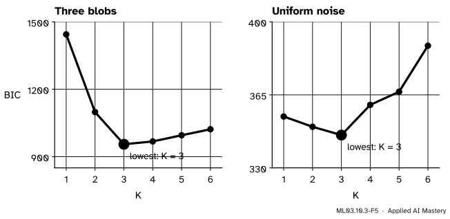
BIC answers a density question. For mixtures, BIC of ML03.4.4 picks the number of Gaussian components that best describe the density. A uniform rectangle is not Gaussian, so several components describe it better than one.
ML03.10.3-F5
BIC of Gaussian mixtures with full covariances. It picks \({K} = {3}\) for the blobs, rightly, and also \({K} = {3}\) for the noise, where three Gaussians simply fit a flat density better than one.
Worked example
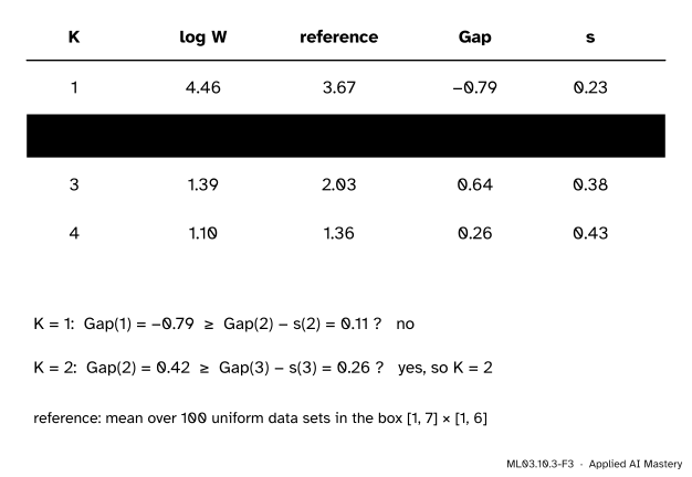
The gap statistic for the nine points, \({K} = {1}\) to \(4\).
The data. The best \(J\) for each \(K\) is known from ML03.1: \(86.222\) (all nine about their mean), \(10.8\), \(4\) (the bridge point alone) and \(3\). Their natural logarithms are
The reference. The bounding box is \({[1, 7] \times [1, 6]}\). One hundred sets of nine uniform points in it, each clustered for every \(K\), give mean values of \({\log W^*_K}\) of \(3.666\), \(2.796\), \(2.029\) and \(1.361\), with \(s_K\) of \(0.226\), \(0.303\), \(0.379\) and \(0.432\). These come from the simulation in the code below; another seed moves them by up to about a tenth, but the choice below stays the same.
The rule. At \({K} = {1}\): is \({-0.791} \ge {0.416 - 0.303} = {0.113}\)? No. At \({K} = {2}\): is \({0.416} \ge {0.643 - 0.379} = {0.264}\)? Yes, so \({\hat K} = {2}\).
ML03.10.3-F3
The gap statistic of the nine points. The largest gap is at \({K} = {3}\), the bridge point alone, but it is within one standard error of \({K} = {2}\), so the rule keeps the simpler answer.
Notice that the gap is largest at \({K} = {3}\). With only nine points the reference is noisy, \(s_3\) is large, and the rule refuses to split off one point without strong evidence.
Code
The gap statistic from scratch, with one set of reference data per draw clustered for every \(K\).
import numpy as npfrom sklearn.cluster import KMeansfrom sklearn.datasets import make_blobsfrom sklearn.metrics import adjusted_rand_score, silhouette_scorefrom sklearn.mixture import GaussianMixturedef W(X, K, seed=0):return KMeans(K, n_init=10, random_state=seed).fit(X).inertia_def gap_statistic(X, Ks, B=20, seed=0): rng = np.random.default_rng(seed) lo, hi = X.min(0), X.max(0) refs = [rng.uniform(lo, hi, size=X.shape) for _ inrange(B)] logW = np.log([W(X, K) for K in Ks]) ref = np.log([[W(R, K) for K in Ks] for R in refs]) gap = ref.mean(0) - logW s = ref.std(0) * np.sqrt(1+1/ B) pick =next((K for i, K inenumerate(Ks[:-1]) if gap[i] >= gap[i +1] - s[i +1]), Ks[-1])return gap, s, pickblobs, _ = make_blobs(n_samples=150, centers=[(0, 0), (4, 4), (8, 0)], cluster_std=0.6, random_state=0)noise = np.random.default_rng(0).uniform(0, 1, size=(150, 2)) * [2, 1]nine = np.array([(1, 1), (2, 1), (1, 2), (2, 2), (6, 5), (7, 5), (6, 6), (7, 6), (4, 4)], float)Ks =list(range(1, 7))for name, X in [("blobs", blobs), ("noise", noise)]: gap, s, pick = gap_statistic(X, Ks)print(f"{name}: gap {np.round(gap, 2)} chosen K = {pick}")gap9, s9, pick9 = gap_statistic(nine, [1, 2, 3, 4], B=100)print("nine points: gap", np.round(gap9, 3), " s", np.round(s9, 3), " chosen K =", pick9)
blobs: gap [-0.08  0.03  1.83  1.65  1.49  1.41]  chosen K = 3
noise: gap [-0.06 -0.1  -0.1  -0.07 -0.02 -0.07]  chosen K = 1
nine points: gap [-0.791  0.416  0.643  0.262]  s [0.226 0.303 0.379 0.432]  chosen K = 2
Now stability, and the silhouette and BIC on the same two data sets.
def stability(X, K, pairs=20, frac=0.8, seed=1): rng = np.random.default_rng(seed); n =len(X); m =int(round(frac * n)); out = []for p inrange(pairs): a, b = rng.choice(n, m, replace=False), rng.choice(n, m, replace=False) shared = np.intersect1d(a, b) fa = KMeans(K, n_init=10, random_state=p).fit(X[a]) fb = KMeans(K, n_init=10, random_state=100+ p).fit(X[b]) out.append(adjusted_rand_score(fa.predict(X[shared]), fb.predict(X[shared])))return np.mean(out)table = {}for name, X in [("blobs", blobs), ("noise", noise)]: sil = [silhouette_score(X, KMeans(K, n_init=10, random_state=0).fit_predict(X)) for K inrange(2, 7)] stab = [stability(X, K) for K inrange(2, 7)] bic = [GaussianMixture(K, n_init=3, random_state=0).fit(X).bic(X) for K inrange(1, 7)] table[name] = (sil, stab, bic)print(f"{name}: best silhouette K = {2+ np.argmax(sil)} ({max(sil):.2f}), "f"most stable K = {2+ np.argmax(stab)} ({max(stab):.2f}), lowest BIC K = {1+ np.argmin(bic)}")
blobs: best silhouette K = 3 (0.81), most stable K = 3 (1.00), lowest BIC K = 3
noise: best silhouette K = 2 (0.48), most stable K = 2 (0.96), lowest BIC K = 3
On the blobs all three agree on \({K} = {3}\). On the noise the silhouette and stability both name \({K} = {2}\) and BIC names \({K} = {3}\); only the gap statistic answers \({K} = {1}\).
Two data sets that fool the gap: one diagonal Gaussian cloud, and three blobs in a triangle.
diagonal cloud: gap [1.01 1.44 1.54 1.59 1.71 1.88]  chosen K = 6
triangle: gap [0.18 0.19 1.26 1.01 0.93 0.85]  chosen K = 1
Explore
ML03.10-X1
Cluster scorecard
Pick a point set and slide \(K\). Each point’s silhouette is drawn as a bar, and the read-out gives the mean silhouette, the Davies-Bouldin index, the adjusted Rand index against the true groups and the stability over 12 pairs of subsamples. Choose uniform noise and look for a \(K\) at which every index says “no clusters”: there is none.
Pitfalls
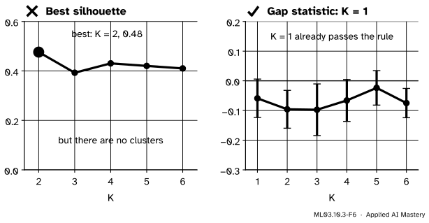
ML03.10.3-F6
Wrong beside right, on the uniform noise. Choosing \(K\) by the best silhouette always returns some \({K} \ge {2}\), here \(2\). The gap statistic compares with noise and stops at \({K} = {1}\).
“The silhouette was highest at K = 2, so the data have two clusters.”
The silhouette ranks values of \(K\) against each other and cannot say “none”. On the noise, \({K} = {2}\) scores \(0.48\), nearly as high as some real clusterings. Before choosing how many clusters, ask whether there are any, with a test that allows \({K} = {1}\).
“The clusters are stable, so they are real.”
Stability shows that the algorithm gives the same answer on similar data. A unique best split of featureless data is reproduced every time: the noise rectangle is stable at \({K} = {2}\). Stability is evidence against an arbitrary \(K\), not proof of structure.
“Pick K by cross-validation, as in supervised learning.”
There is no held-out target to predict. \(W_K\) falls with \(K\) on held-out data too, because more centres fill the space more densely (ESL 14.3.11). That is why the gap statistic, stability and likelihood-based criteria such as BIC exist; each answers its own narrower question, so use more than one and look at the data.
Check yourself
Recall
1. Why can no internal index such as the silhouette conclude that there are no clusters?
Show answer
It is defined only for \({K} \ge {2}\) and scores how good a given partition is. Any data can be partitioned, and the best partition of noise still gets a positive score.
2. What reference data does the gap statistic use in its simplest form?
Show answer
Points drawn uniformly over the range of each feature, that is, in the bounding box of the data, with the same number of points.
3. State the rule that chooses \(K\) from the gap.
Show answer
The smallest \(K\) with \({\mathrm{Gap}(K)} \ge {\mathrm{Gap}(K + 1) - s_{K+1}}\), where \({s_K} = {\mathrm{sd}_K\sqrt{1 + 1/B}}\).
4. How is stability measured in this lesson?
Show answer
By clustering two random 80 percent subsamples with the same \(K\), computing the adjusted Rand index of the two labellings on the points they share, and averaging over 20 pairs.
5. Why does BIC choose \({K} = {3}\) for the uniform rectangle?
Show answer
BIC chooses how many Gaussian components best describe the density. A flat rectangle is not Gaussian, so a few Gaussians side by side fit it better than one, even though there are no groups.
Exercises
1.★ A gap table reads: Gap \(= {0.10, 0.62, 0.58, 0.57}\) for \({K} = {1}\) to \(4\), with \({s} = {0.05, 0.06, 0.07, 0.08}\). Which \(K\) does the rule choose?
Show solution
\({K} = {1}\): is \({0.10} \ge {0.62 - 0.06} = {0.56}\)? No. \({K} = {2}\): is \({0.62} \ge {0.58 - 0.07} = {0.51}\)? Yes. So \({\hat K} = {2}\).
2.★★ For one cluster of three points at \(0\), \(1\) and \(5\) on a line, compute \(D\), the sum of squared distances over all ordered pairs, and check that \({D/(2n)}\) equals the sum of squares about the mean.
Show solution
The unordered pairs have squared distances \(1\), \(25\) and \(16\), which add to \(42\); ordered pairs count each twice, so \({D} = {84}\), and \({D/(2n) = 84/6 = 14}\). The mean is \(2\), and the squares about it are \({4} + {1} + {9} = {14}\). They agree.
3.★★★ Explain why \(B\) reference data sets give the term \({\sqrt{1 + 1/B}}\) in \(s_K\). Treat \({\log W^*_{Kb}}\) as independent draws with standard deviation \(\sigma\), and ignore the randomness of the data’s own \({\log W_K}\).
Show solution
The gap uses the average of \(B\) draws, whose variance is \({\sigma^2/B}\). The question the rule asks is whether the data behave like one more draw from the reference, and one draw varies with variance \(\sigma^2\). The difference between a new draw and an independent estimated mean has variance \({\sigma^2} + {\sigma^2/B} = {\sigma^2(1 + 1/B)}\), so its standard deviation is \({\sigma\sqrt{1 + 1/B}}\). Replacing \(\sigma\) by the sample value \(\mathrm{sd}_K\) gives \(s_K\). With large \(B\) the factor tends to 1; with \({B} = {20}\) it is \(1.025\).
Summary card
First ask whether there are clusters, then how many.
ML03.10.3-F1
Every algorithm returns clusters.
Gap.\({\mathrm{Gap}(K)} = {\overline{\log W^*_K} - \log W_K}\) against uniform data in the box.
Rule. Smallest \(K\) with \({\mathrm{Gap}(K)} \ge {\mathrm{Gap}(K+1) - s_{K+1}}\); it may be 1.
Stability. Mean ARI between fits on overlapping subsamples.
Limits. The gap depends on its reference; stability rewards unique splits; BIC counts Gaussians.
Noise. Silhouette and stability say \({K} = {2}\), BIC \({K} = {3}\), the gap \({K} = {1}\).
Sources and next steps
Sources. Each was opened and checked against this lesson on 15 November 2026.
Robert Tibshirani, Guenther Walther and Trevor Hastie, Estimating the number of clusters in a data set via the gap statistic, Journal of the Royal Statistical Society B 63 (2001), 411 to 423. Section 2 defines \(D_r\) (equation 1), \(W_k\) (equation 2) and the gap (equation 3); Section 3 argues that the uniform distribution is the reference most likely to produce spurious clusters; Section 4 gives the two references, (a) uniform over each feature’s range and (b) a box aligned with the principal components, \({s_k} = {\sqrt{1 + 1/B}\,\mathrm{sd}(k)}\) and the rule “smallest \(k\) such that Gap(\(k\)) ≥ Gap(\({k} + {1}\)) − \(s_{k+1}\)”, and an example on 100 uniform points where the estimate is 1.
Trevor Hastie, Robert Tibshirani and Jerome Friedman, The Elements of Statistical Learning, 2nd edition. Section 14.3.11 explains that \(W_K\) decreases with \(K\) even on an independent test set, so cross-validation cannot choose \(K\), and states the gap rule as equation 14.39 with 20 reference simulations.
Ulrike von Luxburg, Clustering Stability: An Overview, Foundations and Trends in Machine Learning 2 (2010), 235 to 274. Section 2 lists the ways of perturbing the data (subsampling without replacement among them) and of comparing clusterings (on the shared points of overlapping subsamples, after Ben-Hur and colleagues); Section 3.1.1 and its Figure 3.1 show that idealised k-means is stable with a wrong \(K\) unless the data are symmetric.