Read PCA as an encoder that squeezes each example into a few numbers and a decoder that rebuilds it. Derive that the mean squared error of the rebuild is the sum of the dropped eigenvalues, compress the digits, and choose the number of components by cross-validation.
ML03.5.1L2 Intermediate25 minIn review (what this means)
The maths and code on this page are checked by automated tests on every change, but an independent reader has not signed it off yet. Spot a mistake or a confusing step? Tell us.
Write PCA as an encoder y = Q_q-transpose (x - mean) and a decoder x-hat = mean + Q_q y, and compute both by hand for a small data set.
Derive that the mean squared reconstruction error, dividing by n - 1, equals the sum of the discarded eigenvalues.
Read an explained-variance curve and rebuild load_digits from 2, 10 and 30 components.
Choose the number of components by the cross-validated accuracy of a Pipeline that fits PCA on the training folds only.
Use sklearn.decomposition.PCA with transform, inverse_transform and svd_solver=‘randomized’, and spot an outlier that swings the first direction.
The question
Each handwritten digit in load_digits is 64 numbers, one per pixel. A classifier, a clustering algorithm or a plot would all rather have fewer. How few numbers can stand in for a digit, how much of the picture do we lose when we squeeze it, and how do we decide how far to squeeze before we hand the data to a model?
Intuition
Module M03.6 found the principal directions of a cloud: the eigenvectors of its covariance matrix. This lesson turns them into a machine with two halves. The encoder takes a point and writes down only its coordinates along the first \(q\) directions, a short code. The decoder takes the code and rebuilds a point in the full space.
ML03.5.1-F1
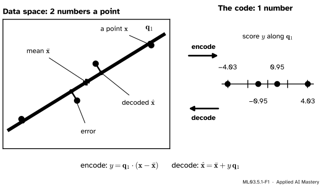
PCA as compression. The encoder keeps one number for each of the four points, its score along the first principal direction. The decoder puts the point back on the line. What is lost is the purple perpendicular gap.
For the four running points the code is a single number per point instead of two, and the rebuilt points all lie on the orange line. Each rebuilt point is the original’s shadow on that line, so the reconstruction error is exactly the perpendicular gap of M03.6.3. That lesson showed that the first principal direction makes those gaps as small as they can be. Here we measure how small, in a form that works for any number of directions, and then put the machine to work in front of a classifier.
Build it up
Step 1. The encoder. Stack the first \(q\) principal directions as the columns of the \({d \times q}\) matrix \(\mat{Q}_q = {[\vect{q}_1 \cdots \vect{q}_q]}\). The code of a point \(\vect{x}\) is
Encoding then decoding is \({\hat{\vect{x}} = \bar{\vect{x}} + \mat{Q}_q\mat{Q}_q\T(\vect{x} - \bar{\vect{x}})}\): the orthogonal projection onto the flat through the mean spanned by the kept directions.
Step 3. What is lost. With all \(d\) directions, \(\mat{Q}\) is square and orthogonal, so \({\mat{Q}\mat{Q}\T = \mat{I}}\) and the rebuild is perfect. Keeping \(q\) of them drops the part of \({\vect{x} - \bar{\vect{x}}}\) that lies along \(\vect{q}_{q+1}, \dots, \vect{q}_d\). That dropped part is the error.
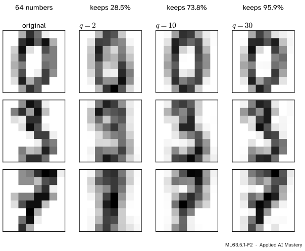
Step 4. Try it on real pictures. Each digit is a point in \(\R^{64}\). Encoding to \(q\) numbers and decoding gives back a 64-pixel picture.
ML03.5.1-F2
Three digits rebuilt from \(q = 2\), \(10\) and \(30\) numbers. Two numbers keep only the rough mass of ink; ten already make each digit readable; thirty are hard to tell from the original.
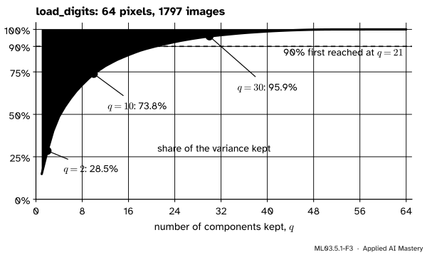
How much is kept is measured by the eigenvalues. The share of the total variance held by the first \(q\) directions, the explained-variance ratio of M03.6.3 added up, is plotted against \(q\) below.
ML03.5.1-F3
The explained-variance curve of the digits. The pink band above the curve is what the decoder cannot rebuild; the next section shows that its height is the sum of the dropped eigenvalues.
The formal statement
NotePCA’s reconstruction error
Let \(\mat{C}\) be the sample covariance of \(\vect{x}_1, \dots, \vect{x}_n\), with eigenvalues \({\lambda_1 \ge \cdots \ge \lambda_d}\) and orthonormal eigenvectors \(\vect{q}_1, \dots, \vect{q}_d\). Encode with \(\mat{Q}_q\) and decode as above. Then
Derivation. Write \(\vect{c}_i = \vect{x}_i - \bar{\vect{x}}\) for the centred point. Because \(\vect{q}_1, \dots, \vect{q}_d\) is an orthonormal basis, \(\vect{c}_i\) is the sum of its pieces along each direction:
The decoder rebuilds only the first \(q\) pieces, so \({\hat{\vect{x}}_i - \bar{\vect{x}}} = {\sum_{j \le q} (\vect{q}_j \cdot \vect{c}_i)\,\vect{q}_j}\), and the error is what remains:
Sum over the points, divide by \(n - 1\) and swap the two sums. For each \(j\), the average squared score is the variance along \(\vect{q}_j\), which M03.6.3 showed is \({\vect{q}_j\T\mat{C}\vect{q}_j}\):
The last step uses \(\mat{C}\vect{q}_j = \lambda_j\vect{q}_j\) and \(\vect{q}_j\T\vect{q}_j = 1\).
Since the eigenvalues add up to the total variance \({\operatorname{tr}(\mat{C})}\), the share of the variance lost is one minus the share kept. That is the pink band of the curve.
Go deeper: no other q directions rebuild better
Take any \({d \times q}\) matrix \(\mat{W}\) with orthonormal columns and use it as encoder and decoder. By the derivation above the error is \({\operatorname{tr}(\mat{C}) - \operatorname{tr}(\mat{W}\T\mat{C}\mat{W})}\), so we must show that \({\operatorname{tr}(\mat{W}\T\mat{C}\mat{W}) \le \lambda_1 + \cdots + \lambda_q}\). Write \(\mat{C} = \sum_j \lambda_j\vect{q}_j\vect{q}_j\T\) (M03.3.3). Then
Each \(a_j\) lies between 0 and 1, because \(\mat{W}\mat{W}\T\) is a projection and cannot lengthen the unit vector \(\vect{q}_j\). And the \(a_j\) add up to \(q\), because \({\sum_j \norm{\mat{W}\T\vect{q}_j}^2}\) is the squared Frobenius norm of \({\mat{W}\T\mat{Q}}\), which equals that of \(\mat{W}\), namely \(q\). A sum \({\sum_j \lambda_j a_j}\) with weights in \([0, 1]\) adding to \(q\) is largest when the weight 1 sits on the \(q\) largest eigenvalues. So the top \(q\) eigenvectors win. Eckart and Young’s theorem (M03.6.1) says the same for any rank-\(q\) reconstruction, not only for orthogonal projections.
Worked example
The four points with \(q = 1\). M03.6.3 found, for \((0, 1)\), \((3, 2)\), \((4, 4)\) and \((7, 5)\), the mean \((3.5, 3)\), the first direction \(\vect{q}_1 \approx {(0.851, 0.526)}\) of slope \(0.618\), and the eigenvalues \({\lambda_1 \approx 11.42}\) and \({\lambda_2 \approx 0.243}\) of \(\mat{C}\).
ML03.5.1-F4
Encode, decode and measure the error for the four points. The average squared error is the eigenvalue that was dropped.
Encode. The first point is \({(-3.5, -2)}\) from the mean, so its score is \({0.851 \times (-3.5) + 0.526 \times (-2)} \approx -4.03\). The other scores are \(-0.95\), \(0.95\) and \(4.03\).
Decode. The first point comes back as \({(3.5, 3) + (-4.03)(0.851, 0.526)} \approx {(0.07, 0.88)}\), and the others as \({(2.69, 2.50)}\), \({(4.31, 3.50)}\) and \({(6.93, 5.12)}\).
Errors. The first point misses by \({(0 - 0.07,\; 1 - 0.88)}\), whose squared length is \({0.0053 + 0.0139} \approx 0.019\). The second misses by about \({(0.31, -0.50)}\), squared length \(0.345\). By symmetry the other two repeat these, and the four add up to \(0.729\).
Average. Dividing by \({n - 1 = 3}\) gives \(0.243\), which is \(\lambda_2\), as the formal statement promised. The exact value is \({\lambda_2 = (35 - 15\sqrt5)/6}\). One number per point keeps \({\lambda_1/(\lambda_1 + \lambda_2)} \approx 97.9\%\) of the variance.
Code
From scratch: the encoder and decoder are two matrix products. We check the error formula on the digits for three values of \(q\).
import numpy as npfrom sklearn.datasets import load_digitsX, labels = load_digits(return_X_y=True) # 1797 images, 64 pixels each, values 0 to 16n =len(X)mean = X.mean(axis=0)lam, Q = np.linalg.eigh((X - mean).T @ (X - mean) / (n -1))lam, Q = lam[::-1], Q[:, ::-1] # largest firstdef encode(X, q):return (X - mean) @ Q[:, :q] # n by q codesdef decode(Y): q = Y.shape[1]return mean + Y @ Q[:, :q].T # back to n by 64 picturesfor q in (2, 10, 30): err = np.sum((X - decode(encode(X, q))) **2) / (n -1)print(f"q = {q:2d}: error {err:7.2f} dropped eigenvalues {lam[q:].sum():7.2f}"f" kept {lam[:q].sum() / lam.sum():.1%}")
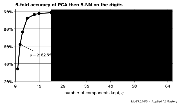
The error and the dropped eigenvalues agree to every printed digit. Now PCA as a preprocessing step: put it in front of a 5-nearest-neighbour classifier (ML01.3) and let cross-validation (ML01.9.3) pick \(q\). Inside a Pipeline, PCA is refitted on the training folds of every split, so the held-out fold never shapes the directions.
Accuracy against the number of components kept. The curve is flat from \(q = 15\) on, so 15 numbers per digit serve the classifier as well as all 64 pixels.
Two components give 62% accuracy. From \(q = 15\) on the accuracy is flat at about 98.3% to 98.6%, the same as with all 64 pixels, so 15 numbers per digit do the job. Note that 95% of the variance needs 29 components: the classifier needs less than the picture.
Last, the library. PCA stores the directions as the rows of components_; transform encodes and inverse_transform decodes. With svd_solver="randomized" it finds only the leading directions, by the randomised SVD of Halko, Martinsson and Tropp, which is much faster when \(q\) is small and the data are large. Its answers are approximate, so we compare with a tolerance.
full = PCA(n_components=10).fit(X)fast = PCA(n_components=10, svd_solver="randomized", random_state=0).fit(X)codes = full.transform(X) # 1797 by 10back = full.inverse_transform(codes) # 1797 by 64print("library error:", round(np.sum((X - back) **2) / (n -1), 2))print("largest relative gap, randomized vs full:",f"{np.max(np.abs(fast.explained_variance_ / full.explained_variance_ -1)):.1e}")
library error: 314.69
largest relative gap, randomized vs full: 3.4e-06
The library’s error matches the hand-built one, and its explained_variance_ holds \(\lambda_1, \dots, \lambda_{10}\). The rows of components_ may differ from our columns of \(\mat{Q}\) by a sign, which changes nothing: \(\mat{Q}_q\mat{Q}_q\T\) is the same either way.
Explore
ML03.5-X1
Variance and error
Turn the line with the slider, or drag its handle, and watch the variance along the line and the mean squared error trade places while their sum stays fixed. Press snap to the first direction, then try the round cloud and the cloud with one outlier; standardise and whiten reshape the cloud first, which the next lesson explains.
Pitfalls
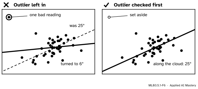
ML03.5.1-F6
Wrong beside right. One reading far from the cloud turns the first direction by almost 20 degrees, because squared distances give it a large say.
“PCA describes the bulk of the data, so a stray point cannot matter much.”
Variance is a mean of squared distances, so one point far away carries the weight of many near ones. In the figure, the point \((-4.5, 3.2)\) alone turns the first direction of the 40-point cloud from \(25°\) to \(6°\). Look at the scores (or at the reconstruction error of each point) before trusting the directions, and set aside or investigate points that sit far out. ML03.9 turns this reconstruction error into an anomaly score.
“I fitted PCA on the whole data set first, then cross-validated the classifier.”
Then every held-out fold helped choose the directions, and the accuracy you report is a little optimistic: the leakage of ML01.2.4. Put PCA inside the Pipeline, as in the code above, so that it is refitted on the training folds alone.
“Keep enough components for 95% of the variance.”
A variance threshold measures how well the pictures are rebuilt, not how well a model predicts. On the digits, 95% needs 29 components while the classifier is already as good as it gets with 15. And the variance a task needs may sit in a small direction (the discriminant directions of ML02.9.4 make the point). When PCA feeds a model, choose \(q\) by validating the model.
Check yourself
Recall
1. What do the encoder and the decoder of PCA compute?
Show answer
The encoder gives the code \({\vect{y} = \mat{Q}_q\T(\vect{x} - \bar{\vect{x}})}\), the scores along the first \(q\) directions. The decoder gives \({\hat{\vect{x}} = \bar{\vect{x}} + \mat{Q}_q\vect{y}}\).
2. What is the mean squared reconstruction error, dividing by \(n - 1\), when \(q\) directions are kept?
Show answer
The sum of the dropped eigenvalues, \({\lambda_{q+1} + \cdots + \lambda_d}\).
3. Why is the reconstruction perfect when \(q = d\)?
Show answer
\(\mat{Q}\) is then square and orthogonal, so \({\mat{Q}\mat{Q}\T = \mat{I}}\) and \({\hat{\vect{x}} = \bar{\vect{x}} + (\vect{x} - \bar{\vect{x}}) = \vect{x}}\).
4. Why must PCA sit inside the Pipeline when \(q\) is chosen by cross-validation?
Show answer
So that it is fitted on the training folds only. Fitted on all the data, the held-out folds would help choose the directions, and the score would leak.
5. What does svd_solver="randomized" trade, and when is it worth it?
Show answer
It gives up exactness for speed: it finds only the leading directions, approximately. It pays off when the data are large and \(q\) is much smaller than \(d\).
Exercises
1.★ A data set in \(\R^4\) has covariance eigenvalues \(6\), \(3\), \(0.6\) and \(0.4\). What share of the variance does \(q = 2\) keep, and what is its mean squared reconstruction error?
Show solution
The total is \({6 + 3 + 0.6 + 0.4} = 10\). Keeping two directions holds \({9/10} = 90\%\). The error, dividing by \(n - 1\), is the sum of the dropped eigenvalues, \({0.6 + 0.4} = 1\), which is the missing \(10\%\) of the total.
2.★★ For the four points, encode and decode with the second direction \({\vect{q}_2 \approx (0.526, -0.851)}\) alone. What is the mean squared error, and why is it so much larger?
Show solution
By the derivation, keeping only \(\vect{q}_2\) drops \(\vect{q}_1\), so the error is \({\lambda_1 \approx 11.42}\). Check one point: \((0, 1)\) is \({(-3.5, -2)}\) from the mean, with score \({0.526 \times (-3.5) + (-0.851)(-2)} \approx -0.14\) along \(\vect{q}_2\), so its rebuild is \({(3.5, 3) - 0.14\,(0.526, -0.851)} \approx (3.43, 3.12)\), far from \((0, 1)\). The direction kept is the one along which the points barely differ, so almost everything is lost.
3.★★★ Show that the codes are uncorrelated and that the sample variance of code \(j\) is \(\lambda_j\): that is, \({\frac{1}{n-1}\sum_i \vect{y}_i\vect{y}_i\T}\) is the diagonal matrix of \({\lambda_1, \dots, \lambda_q}\).
Show solution
With \(\vect{c}_i = \vect{x}_i - \bar{\vect{x}}\) and \(\vect{y}_i = \mat{Q}_q\T\vect{c}_i\),
Entry \((j, k)\) is \({\vect{q}_j\T\mat{C}\vect{q}_k} = {\lambda_k\,\vect{q}_j\T\vect{q}_k}\), which is \(\lambda_j\) when \(j = k\) and 0 otherwise, since the eigenvectors are orthonormal. The codes also have mean zero, because the \(\vect{c}_i\) add up to zero, so this matrix is their covariance.
Summary card
PCA is an encoder to \(q\) numbers and a decoder back; the error is what the dropped eigenvalues held.
Choosing \(q\). For pictures, the explained-variance curve; for a model, cross-validation with PCA inside the Pipeline.
Sources and next steps
Sources. Each was opened and checked against this lesson on 15 November 2026.
Christopher M. Bishop, Pattern Recognition and Machine Learning (Springer, 2006; full PDF from Microsoft Research). Section 12.1.2, the minimum-error formulation: the distortion measure (12.11) is the mean squared distance between each point and its approximation, and its minimum (12.18) is the sum of the eigenvalues of the discarded directions. Bishop divides by \(N\) rather than \(n - 1\).
scikit-learn 1.9, sklearn.decomposition.PCA: explained_variance_ uses \(n - 1\) degrees of freedom and equals the largest eigenvalues of the covariance matrix; inverse_transform transforms data back to the original space; svd_solver="randomized" runs the randomised SVD of Halko, Martinsson and Tropp (SIAM Review 53, 2011). The User Guide, Section 2.5.1.3 explains when the randomised solver pays off.
scikit-learn 1.9, sklearn.datasets.load_digits: 1797 images of 8 by 8 pixels, 64 features with integer values from 0 to 16, ten classes.