Take the hills of a kernel density estimate as clusters. Derive the gradient of a Gaussian estimate, show that moving a point to the kernel-weighted mean of the data is a gradient-ascent step with an adaptive size, and cluster the six values and seeded blobs from scratch and with MeanShift.
ML03.8.4L2 Intermediate25 minIn review (what this means)
The maths and code on this page are checked by automated tests on every change, but an independent reader has not signed it off yet. Spot a mistake or a confusing step? Tell us.
Explain how the modes of a kernel density estimate define clusters, and why the bandwidth sets their number.
Derive the gradient of a Gaussian kernel estimate and show that the mean-shift step equals h squared times the gradient of its logarithm.
Run mean shift by hand for a few steps on the six values and from scratch in NumPy on blobs in the plane.
Use sklearn.cluster.MeanShift with estimate_bandwidth, and compare mean shift with DBSCAN and with k-means.
The question
k-means needs to be told how many clusters to find. A kernel density estimate already shows where the data crowd: its hills. If every point simply walked uphill until it could climb no further, the points that met at the same summit would form a cluster. How do we climb a density we only know as a sum of bumps, and who decides how many summits there are?
From the last lesson
1. Write the Gaussian kernel estimate in \({\R^d}\) with one bandwidth \(h\).
2. Why standardise features before using a single bandwidth?
Show answer
Because a bandwidth is a distance in each feature’s units; after standardising, one \(h\) means the same width in every direction.
Intuition
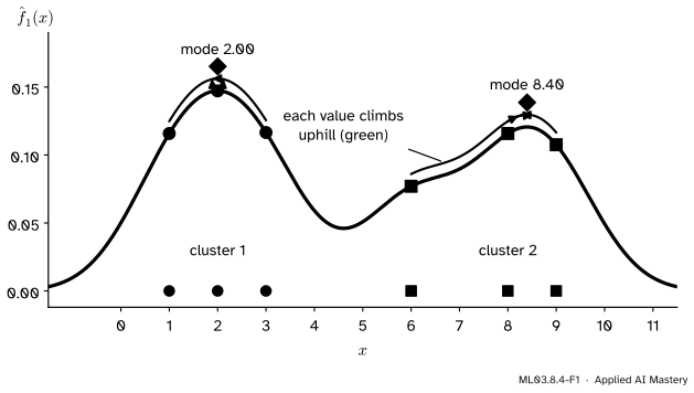
Take the kernel estimate of the six values 1, 2, 3, 6, 8 and 9 with \({h = 1}\) from lesson ML03.8.1. It has two hills. Put each value on the curve and let it climb.
ML03.8.4-F1
Mean shift on the six values. Each value climbs the estimate to the top of its hill, a mode. Values that reach the same mode form a cluster: {1, 2, 3} and {6, 8, 9}.
Three things in the picture are the whole method. A mode is a local maximum of the estimate, the top of a hill. Each point climbs to the mode whose hill it stands on. And the number of clusters is the number of modes that some point reaches, which the bandwidth decides: narrow bumps make many small hills, wide bumps make few. The value 6 shows a subtlety: it sits on a shoulder, not on a hill of its own, so it walks all the way to the hill at 8.4.
Build it up
Step 1. Climbing needs the slope. Gradient ascent, the mirror image of the gradient descent of ML01.5, moves a point a small step in the direction in which the function rises fastest, the gradient. For a sum of bumps, the gradient is a sum of the bumps’ slopes, so it is easy to compute.
Step 2. Gradient ascent needs a step size. Too small and the climb takes for ever; too large and it overshoots the summit. The happy discovery behind mean shift is that, for a kernel estimate, there is a step size that needs no tuning.
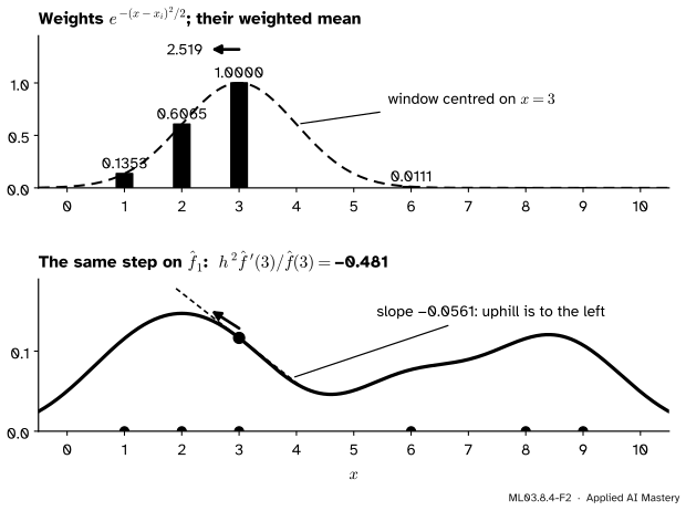
Step 3. Move to the weighted mean. Give each data point a weight that is large when it is close to the current position: its kernel value. Then move to the weighted mean of the data. Points on the uphill side are more numerous or closer, so they pull harder, and the mean lies uphill.
ML03.8.4-F2
One mean-shift step from \({x = 3}\) with \({h = 1}\). Top: the weighted mean of the data is 2.519. Bottom: the same move is a step up the estimate, of size \({h^2}\) times the slope over the height.
The formal statement
Take the Gaussian estimate in \({\R^d}\) and write \({w_i(\vect{x}) = e^{-\norm{\vect{x} - \vect{x}_i}^2/(2h^2)}}\) for the weight of data point \(i\), and \({c = 1/\big(n (2\pi h^2)^{d/2}\big)}\) for the constant, so that
\[
\hat f(\vect{x}) = c \sum_{i=1}^n w_i(\vect{x}) .
\]
The gradient. By the chain rule, the gradient of \({-\norm{\vect{x} - \vect{x}_i}^2/(2h^2)}\) is \({(\vect{x}_i - \vect{x})/h^2}\), so \({\nabla w_i(\vect{x}) = w_i(\vect{x})\,(\vect{x}_i - \vect{x})/h^2}\). Summing,
It is a gradient-ascent step on \(\hat f\) with step size \({h^2/\hat f(\vect{x})}\).
The step size adapts by itself. Where the density is low, \({1/\hat f}\) is large and the step is long: a point in an empty region is moved quickly towards the data. Near a mode the gradient shrinks to zero, so the steps shrink too, and the point settles. It stops exactly where \({\vect{m} = \vect{0}}\), that is where \({\nabla \hat f = \vect{0}}\). Comaniciu and Meer proved that for kernels like the Gaussian the sequence of positions converges and the density rises at every step, which is why no learning rate is needed.
The algorithm. Start a copy of the step at every data point and repeat it until the moves are tiny. Points whose end positions agree, within a tolerance much smaller than \(h\), form one cluster, and their common end position is its centre. The bandwidth sets how many hills there are, and so how many clusters.
ML03.8.4-F3
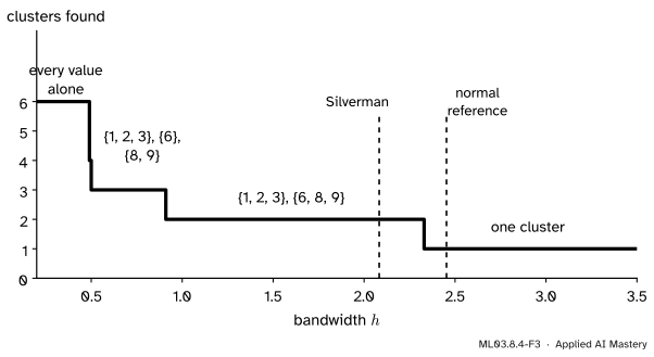
The number of clusters on the six values as the bandwidth grows: 6, then briefly 4, then 3, 2 and 1. Silverman’s bandwidth (2.08) gives two clusters; the normal reference rule (2.45) merges everything.
Go deeper: the flat kernel of MeanShift, and the shadow of a kernel
scikit-learn’s MeanShift uses a flat kernel: the weight is 1 for data within distance \(h\) and 0 beyond, so each step moves to the plain mean of the points within the window. Comaniciu and Meer show the general rule: mean shift with weights from a kernel \(G\) climbs the estimate made with a kernel \(K\) whose profile has \(G\)’s profile as its negative derivative, called the shadow of \(G\). For the Gaussian, the shadow is the Gaussian itself, which is the derivation above. For the flat kernel, the shadow is the Epanechnikov kernel: in one dimension, \({\tfrac{d}{dx}(1 - x^2/h^2) = -2x/h^2}\) on the window and 0 outside, so the gradient of an Epanechnikov estimate is again proportional to the plain mean of the points in the window minus \(x\). With a flat kernel the windows can contain only finitely many different sets of points, so the procedure stops after finitely many steps.
Worked example
Run mean shift from \({x = 3}\) on the six values with \({h = 1}\).
Step 1. The weights \({e^{-(3 - x_i)^2/2}}\) are \({e^{-2} = 0.1353}\) for 1, \({e^{-0.5} = 0.6065}\) for 2, \({e^0 = 1}\) for 3, \({e^{-4.5} = 0.0111}\) for 6, and less than \({10^{-5}}\) for 8 and 9. Computed before rounding, their sum is 1.7530, and the weighted sum of the values is
so the new position is \({4.4150/1.7530 = 2.519}\), a move of \({-0.481}\).
ML03.8.4-F4
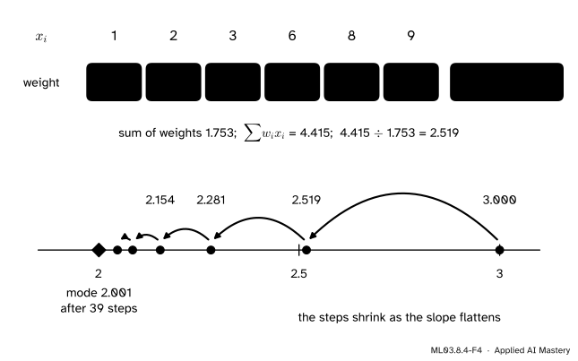
The worked example. One step is a weighted mean; repeated steps shrink as the point nears the mode.
The same step as gradient ascent. The estimate at 3 is \({\hat f(3) = 0.1166}\) and its slope is \({\hat f'(3) = -0.0561}\), so \(h^2 \hat f'(3)/\hat f(3) = {-0.0561/0.1166} = -0.481\): the same move, as the derivation promised.
The next steps. From 2.519 the weights shift towards 1 and 2 and the next mean is 2.281; then 2.154, 2.085, 2.048. Each move is roughly half the one before, because the slope flattens near the top. After 39 steps the moves are below \({10^{-10}}\) and the point rests at the mode 2.001. Starting from 1 and 2 leads to the same mode; starting from 6, 8 and 9 leads to the other mode, 8.397. Two clusters, {1, 2, 3} and {6, 8, 9}, the same split that the Gaussian mixture of ML03.4 settles on.
Code
From scratch on a line first: every value climbs, then end points closer than \({10^{-3}}\) are merged.
import numpy as npx = np.array([1, 2, 3, 6, 8, 9], dtype=float)def climb(start, data, h, tol=1e-10, max_steps=20_000): z, path = start, [start]for _ inrange(max_steps): w = np.exp(-((z - data) / h) **2/2) new = (w * data).sum() / w.sum() # the mean-shift step path.append(new)ifabs(new - z) < tol:break z = newreturn np.array(path)def mean_shift_1d(data, h, merge=1e-3): ends = [climb(v, data, h)[-1] for v in data] modes, labels = [], []for e in ends: hit = [k for k, m inenumerate(modes) ifabs(e - m) < merge]if hit: labels.append(hit[0])else: modes.append(e) labels.append(len(modes) -1)return np.array(modes), np.array(labels)path = climb(3.0, x, 1.0)modes, labels = mean_shift_1d(x, 1.0)print("from 3:", path[:6].round(3), "... ->", round(path[-1], 4), f"after {len(path) -1} steps")print("modes:", modes.round(3), " labels:", labels)print("clusters for h = 0.3, 0.75, 1, 2.083, 2.453:", [len(mean_shift_1d(x, h)[0]) for h in (0.3, 0.75, 1.0, 2.083, 2.453)])
from 3: [3.    2.519 2.281 2.154 2.085 2.048] ... -> 2.0013 after 39 steps
modes: [2.001 8.397]  labels: [0 0 0 1 1 1]
clusters for h = 0.3, 0.75, 1, 2.083, 2.453: [6, 3, 2, 2, 1]
The last assertion checks the derivation numerically: \({h^2 \hat f'(3)/\hat f(3)}\) equals the first move exactly. Now the plane: three seeded blobs, every point moved at once with one \({n \times n}\) matrix of weights per step.
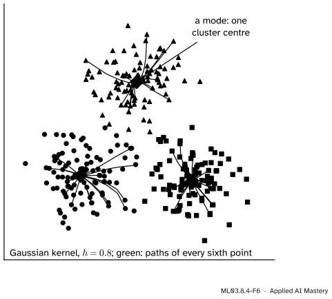
from sklearn.datasets import make_blobsfrom sklearn.metrics import adjusted_rand_scoreX, truth = make_blobs(300, centers=[(0, 0), (4, 0), (2, 3.5)], cluster_std=0.8, random_state=0)def mean_shift(X, h, tol=1e-6, max_steps=500): Z = X.copy()for step inrange(1, max_steps +1): W = np.exp(-((Z[:, None, :] - X[None, :, :]) **2).sum(axis=2) / (2* h * h)) # n x n weights new = W @ X / W.sum(axis=1, keepdims=True)if np.abs(new - Z).max() < tol:return new, step Z = newreturn Z, max_stepsends, steps = mean_shift(X, h=0.8)centres, ours = [], np.zeros(len(X), dtype=int)for i, e inenumerate(ends): hit = [k for k, c inenumerate(centres) if np.linalg.norm(e - c) <0.4]if hit: ours[i] = hit[0]else: centres.append(e) ours[i] =len(centres) -1print(f"{steps} steps, {len(centres)} clusters of sizes {np.bincount(ours).tolist()}")print("centres:", np.round(centres, 2).tolist())print(f"adjusted Rand index against the true blobs: {adjusted_rand_score(truth, ours):.3f}")
35 steps, 3 clusters of sizes [102, 101, 97]
centres: [[-0.09, 0.09], [3.88, -0.09], [1.91, 3.43]]
adjusted Rand index against the true blobs: 0.941
ML03.8.4-F6
Mean shift in the plane with \({h = 0.8}\). Every point’s path ends at one of three modes, and the points sharing a mode share a shape.
scikit-learn’s MeanShift uses a flat kernel, so its bandwidth is a radius, not a standard deviation. Left out, the bandwidth is set by estimate_bandwidth, which averages each point’s distance to its \({\lfloor 0.3\,n \rfloor}\)-th nearest neighbour (counting the point itself). For comparison, DBSCAN (ML03.3) on the same points.
from sklearn.cluster import DBSCAN, MeanShift, estimate_bandwidthradius = estimate_bandwidth(X) # quantile=0.3 by defaultlibrary = MeanShift(bandwidth=radius).fit(X)print(f"estimate_bandwidth: {radius:.3f}; MeanShift found {len(library.cluster_centers_)} clusters,"f" sizes {sorted(np.bincount(library.labels_).tolist())}")print("same clusters as ours:", adjusted_rand_score(ours, library.labels_) ==1.0)db = DBSCAN(eps=0.6, min_samples=5).fit(X)print(f"DBSCAN: {len(set(db.labels_)) -1} clusters, {np.sum(db.labels_ ==-1)} noise points,"f" adjusted Rand {adjusted_rand_score(truth, db.labels_):.3f}")print("estimate_bandwidth on the six values:", estimate_bandwidth(x[:, None]))
estimate_bandwidth: 2.106;  MeanShift found 3 clusters, sizes [97, 101, 102]
same clusters as ours: True
DBSCAN: 3 clusters, 10 noise points, adjusted Rand 0.863
estimate_bandwidth on the six values: 0.0
The flat kernel with radius 2.106 and our Gaussian with standard deviation 0.8 give exactly the same three clusters. DBSCAN finds the same three dense regions but labels 10 sparse points as noise, which mean shift never does: it has a density estimate, and every point, however isolated, has an uphill direction. The last line is a warning, taken up below.
The cost. Every step compares every point with every data point: \({n^2}\) kernel values per iteration, 90,000 here, for about 35 iterations. On large data that is the bottleneck, and MeanShift eases it with a ball tree and with bin_seeding=True, which starts from a coarse grid of points instead of from all of them.
Explore
This module’s interactive, the bandwidth explorer, lives in ML03.8.2. Its read-out counts the hills of the estimate, and each hill is one cluster that mean shift would find: slide the bandwidth across 0.5, 0.9 and 2.3 with the Gaussian kernel and watch the count change as in the step plot above.
Pitfalls
ML03.8.4-F5
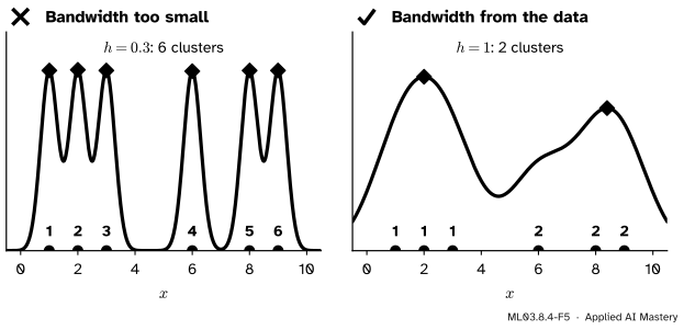
Wrong beside right. With \({h = 0.3}\) every value is its own hill and its own cluster; with \({h = 1}\) the hills, and the clusters, are the two groups.
“Mean shift finds the number of clusters by itself.”
It finds the number of hills, and the bandwidth makes the hills. On the six values the count runs 6, 4, 3, 2, 1 as \(h\) grows. Mean shift trades the choice of \(K\) for the choice of \(h\), which is easier to reason about (lesson ML03.8.2), but it is still a choice.
“estimate_bandwidth always gives a usable bandwidth.”
On the six values it returns 0.0. With the default quantile 0.3 it uses the \({\lfloor 0.3 \cdot 6 \rfloor = 1}\)st nearest neighbour, and the nearest neighbour of a point is the point itself. On small samples, set the bandwidth yourself or raise quantile.
“A bandwidth from KernelDensity can be passed straight to MeanShift.”
MeanShift’s bandwidth is the radius of a flat window, KernelDensity’s is the standard deviation of a Gaussian bump. On the blobs, a radius of 2.106 and a standard deviation of 0.8 gave the same clusters. Using 0.8 as a radius would make the windows far too small.
Check yourself
Recall
1. What is a mode, and how does mean shift turn modes into clusters?
Show answer
A local maximum of the density estimate. Each data point climbs to a mode, and the points that reach the same mode form one cluster, with the mode as its centre.
2. Write the mean-shift step for the Gaussian kernel.
4. Why are mean-shift steps long in sparse regions and short near a mode?
Show answer
The step size \({h^2/\hat f(\vect{x})}\) is large where the density is low, and near a mode the gradient itself goes to zero.
5. What does each iteration of mean shift cost, and how does sklearn’s MeanShift differ from the Gaussian version?
Show answer
About \({n^2}\) kernel evaluations when every point moves. MeanShift uses a flat kernel of radius bandwidth, which climbs an Epanechnikov estimate.
Exercises
1.★ Do one mean-shift step from \({x = 9}\) on the six values with \({h = 1}\).
Show solution
The weights \({e^{-(9 - x_i)^2/2}}\) are about 0 for 1, 2 and 3, \({e^{-4.5} = 0.0111}\) for 6, \({e^{-0.5} = 0.6065}\) for 8 and 1 for 9. The weighted mean is
2.★★ Show that a single data point is a fixed point of mean shift whatever \(h\) is, and that two points at 0 and \(a\) give one mode at \({a/2}\) when \({a < 2h}\). (Hint: the estimate is a mixture of two equal normals; look at its second derivative at the midpoint.)
Show solution
With one point, the weighted mean of the data is that point, so the step returns it. For two points, by symmetry the midpoint \({a/2}\) is always a stationary point. Shift so that the points sit at \({\pm b}\) with \({b = a/2}\). Each bump is proportional to \({e^{-(x \mp b)^2/(2h^2)}}\), whose second derivative at 0 is proportional to \({(b^2/h^2 - 1)\,e^{-b^2/(2h^2)}/h^2}\). Both bumps give the same value, so the sum is curved downwards at 0, a maximum, when \({b < h}\), that is \({a < 2h}\). A sum of two equal bumps then has no other peak, so it is the only mode and both points climb to \({a/2}\). When \({a > 2h}\) the midpoint is a dip and each point keeps its own mode.
3.★★★ In one dimension with the Gaussian kernel, suppose \({\hat f'(x) > 0}\) and \({\hat f}\) is concave from \(x\) up to \({x^*}\), the first point to the right of \(x\) where \({\hat f' = 0}\). Show that one mean-shift step does not lower the density, and explain why a fixed learning rate would not give this guarantee.
Show solution
Write the step map as \({T(z) = \sum_i w_i(z)\,x_i / \sum_i w_i(z)}\) and the step as \({x' = T(x) = x + \delta}\) with \({\delta = h^2 \hat f'(x)/\hat f(x) > 0}\).
The step cannot pass the top. Since \({w_i'(z) = w_i(z)(x_i - z)/h^2}\), the quotient rule gives \({T'(z) = \big(\overline{x^2} - \bar x^2\big)/h^2}\), where the bars are averages with weights \({w_i(z)}\). That is a weighted variance over \({h^2}\), so \({T' \ge 0}\) and \(T\) is increasing. At \({x^*}\) the gradient is 0, so the mean-shift vector is 0 and \({T(x^*) = x^*}\). Hence \({x' = T(x) \le T(x^*) = x^*}\).
The slope at the new point is not negative.\({\hat f'}\) has no zero between \(x\) and \({x^*}\) and is positive at \(x\), so \({\hat f'(x') \ge 0}\).
The density rises. A concave function lies below its tangent lines, so \({\hat f(x) \le \hat f(x') + \hat f'(x')(x - x')}\), that is
A fixed learning rate \(\eta\) moves by \({\eta\,\hat f'(x)}\) whatever the shape nearby, and on a steep slope that can jump past the top and down the other side. Mean shift’s step is tied to the data through \(T\), which can never carry a point past a mode. Comaniciu and Meer’s Theorem 1 proves the general statement: the density rises at every step.
Summary card
Mean shift: move every point to the kernel-weighted mean until it reaches a mode.
Why it climbs:\({\vect{m}(\vect{x}) = h^2\,\nabla \hat f/\hat f}\), gradient ascent with an adaptive step.
Clusters: points with the same mode; the bandwidth sets how many.
In code:MeanShift(bandwidth=estimate_bandwidth(X)), a flat kernel; about \({n^2}\) work per iteration.
Sources and next steps
Sources. Each was opened and checked against this lesson on 15 November 2026.
D. Comaniciu and P. Meer, Mean Shift: A Robust Approach Toward Feature Space Analysis, IEEE Transactions on Pattern Analysis and Machine Intelligence 24(5), May 2002, pages 603 to 619. Section 2.1: the mean-shift vector (equation 17) is proportional to the normalised density gradient (19), “an adaptive gradient ascent method”, and the Epanechnikov kernel is the shadow of the uniform kernel; Section 2.2: the sequence (20) and Theorem 1, convergence with a monotonically increasing density, and finite convergence for the uniform kernel.
scikit-learn, MeanShift: “mean shift clustering using a flat kernel”, bandwidth estimated by estimate_bandwidth when not given, bin_seeding, cluster_all, and complexity tending to \({O(T n^2)}\) in higher dimensions; and estimate_bandwidth, with quantile=0.3 by default and time at least quadratic in the number of samples.
L. Wasserman, Density Estimation, lecture notes for 36-708, Carnegie Mellon University. Section 8 on derivatives of the density estimate, with mode-based clustering: estimate the density, find its modes, and associate a cluster with each mode.
Next. ML03.9, Anomaly detection, turns the estimate around: instead of climbing to where the density is high, it flags the points where it is low.