Agglomerative clustering starts with every point alone and keeps merging the two closest clusters. Run it by hand on six values, read the dendrogram that records every merge, and build it from scratch with a distance matrix.
ML03.2.1L2 Intermediate25 minIn review (what this means)
The maths and code on this page are checked by automated tests on every change, but an independent reader has not signed it off yet. Spot a mistake or a confusing step? Tell us.
Describe agglomerative clustering: start with n clusters of one point and merge the two closest clusters n − 1 times, recording each merge height.
Read a dendrogram from the leaves to the root, and read off the clusters for any number K.
Run single-linkage merging by hand on a small set of values and prove that its merge heights never decrease.
Implement agglomerative clustering from scratch with a distance matrix updated after each merge, and count its cost of about n³/6 comparisons.
The question
k-means needs the number of clusters before it starts. A biologist sorting specimens, or a shop sorting its customers, often does not know that number, and would like groups within groups: species within genera, small segments within large ones. Can one run of an algorithm give the answer for every number of clusters at once?
Intuition
Start with every point in a cluster of its own. Find the two clusters that are closest and merge them. Now there is one cluster fewer. Repeat until a single cluster holds everything. Write down each merge, and how far apart the two clusters were when they merged.
ML03.2.1-F1
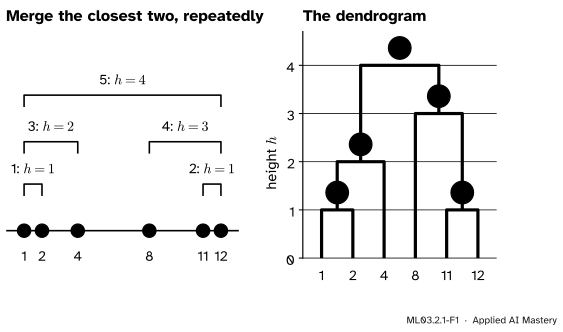
Merging from the bottom up on the six values. Each bracket on the left is one merge; the dendrogram on the right draws each merge as a join at its height \(h\), the distance between the two clusters it joined.
The record of all the merges is a tree. Its leaves are the points; each join is a merge; the height of a join is how far apart the two clusters were. Read upwards, it tells the story of the merging. Read across at any level, it gives a clustering: below height 2.5 the six values form three clusters, {1, 2, 4}, {8} and {11, 12}; below height 3.5 they form two. One tree holds every clustering, from six clusters of one at the bottom to a single cluster at the top.
This is agglomerative (bottom-up) hierarchical clustering. Its other half, divisive (top-down) clustering, which keeps splitting, returns in lesson ML03.2.4.
Build it up
Step 1. Every point is a cluster. With \(n\) points there are \(n\) clusters, each of one point.
Step 2. Decide what “closest clusters” means. Between two points we use the distance \(d_{ij}\) of ML01.3. Between two clusters we need a rule. In this lesson we use the simplest one, single linkage: the distance between clusters \(A\) and \(B\) is the distance between their closest pair of members, one from each. The next lesson meets the alternatives.
Step 3. Merge the closest pair and record the height. The merge height \(h\) is the distance between the two clusters at the moment they merge. One merge turns \(K\) clusters into \({K - 1}\).
Step 4. Repeat. After \({n - 1}\) merges there is one cluster, and the run stops. There is no starting guess and nothing random: the same data always give the same merges (up to ties).
ML03.2.1-F2
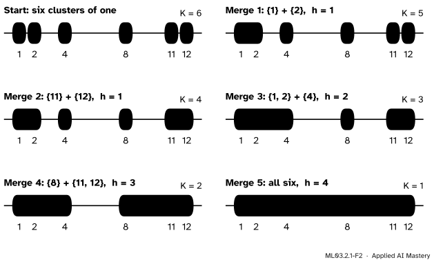
Single linkage on the six values, one merge per panel. The yellow capsule is the cluster just made; \(K\) counts the clusters left.
Two things stand out. First, the clusters for \({K = 3}\) are unions of the clusters for \({K = 4}\), and so on up: each level is made by gluing two clusters of the level below. The clusterings are nested, which is what “hierarchical” means. Second, the heights 1, 1, 2, 3, 4 never go down. That is no accident, and it is what lets the tree be drawn with every join above the joins beneath it.
The formal statement
NoteAlgorithm: agglomerative clustering
Input: points \({\vect{x}_1, \dots, \vect{x}_n}\) (or just their distances \(d_{ij}\)) and a linkage \({D(A, B)}\), the distance between two clusters.
Start with the \(n\) clusters \({\{1\}, \{2\}, \dots, \{n\}}\).
Repeat \({n - 1}\) times: find the pair of current clusters \({A \neq B}\) with the smallest \({D(A, B)}\); replace them by \(A \cup B\); record the merge and its height \({h = D(A, B)}\).
Output: the \({n - 1}\) merges and their heights, drawn as a dendrogram.
A dendrogram is a tree with \(n\) leaves, one per point, and \({n - 1}\) joins, one per merge, each drawn at its merge height. To get \(K\) clusters, stop after \({n - K}\) merges; equivalently, cut the tree with a horizontal line between the \({(n - K)}\)-th and the \({(n - K + 1)}\)-th merge heights. The clusters are the groups of leaves still joined below the line. Lesson ML03.2.3 is about where to cut.
Merge heights never decrease under single linkage. Suppose merge \(t\) joins \(A\) and \(B\) at height \({h_t = D_{\min}(A, B)}\). Because it was the smallest distance between any two clusters, every other pair of clusters is at least \(h_t\) apart. After the merge, only the distances to the new cluster are new, and for any other cluster \(C\)
The second line splits the minimum over \(A \cup B\) into a minimum over \(A\) and one over \(B\). The last line holds because both \({D_{\min}(A, C)}\) and \({D_{\min}(B, C)}\) were at least \(h_t\). So every distance between clusters after merge \(t\) is at least \(h_t\), and the next merge height obeys \({h_{t+1} \ge h_t}\). The middle line is also the update rule the code will use: the new cluster’s distance to \(C\) is the smaller of its two parts’ distances.
What a run costs. Done directly, each merge scans all pairs of current clusters for the smallest distance. With \(m\) clusters there are \({m(m - 1)/2}\) pairs, and \(m\) runs from \(n\) down to 2, so the number of distances examined is
The first equality is the hockey-stick identity: each term \({m(m - 1)/2}\) is \(\binom{m}{2}\), and adding \(\binom{m}{2}\) from \({m = 2}\) to \(n\) gives \({\binom{n+1}{3}}\). So the direct method takes about \({n^3/6}\) steps, and it needs the \({n(n - 1)/2}\) distances in memory. For \({n = 10{,}000}\) points that is about \({1.7 \times 10^{11}}\) comparisons and 50 million distances, 400 MB in double precision. Faster algorithms exist (lesson ML03.2.4), but the memory for all the distances remains.
Worked example
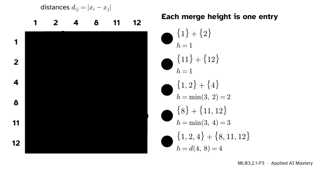
Single linkage on the values 1, 2, 4, 8, 11, 12. The distance between two values is the gap between them, \({d_{ij} = |x_i - x_j|}\). Write all fifteen in a table and the work is a hunt for the smallest entry.
ML03.2.1-F3
The distance matrix of the six values. Under single linkage every merge height is one entry of this table: the gap between the closest members of the two clusters.
The smallest entries are the two 1s. Merge \(\{1\}\) and \(\{2\}\) at \({h = 1}\) (ties are broken by taking the first in the table).
Merge \(\{11\}\) and \(\{12\}\) at \({h = 1}\).
Now the clusters are \({\{1, 2\}}\), \(\{4\}\), \(\{8\}\) and \({\{11, 12\}}\). Their single-linkage distances are \({D(\{1,2\}, \{4\}) = \min(3, 2) = 2}\), \({D(\{4\}, \{8\}) = 4}\), \({D(\{8\}, \{11,12\})}\)\({= \min(3, 4)}\)\({= 3}\), and larger ones further apart. The smallest is 2: merge \({\{1, 2\}}\) with \(\{4\}\) at \({h = 2}\).
Left: \({\{1, 2, 4\}}\), \(\{8\}\), \({\{11, 12\}}\). Now \({D(\{1,2,4\}, \{8\}) = 4}\) and \({D(\{8\}, \{11,12\}) = 3}\). Merge \(\{8\}\) with \({\{11, 12\}}\) at \({h = 3}\).
The last two clusters are closest at the pair 4 and 8, so they merge at \({h = 4}\).
The heights are 1, 1, 2, 3, 4. Cutting the tree anywhere between 3 and 4 leaves the two clusters \({\{1, 2, 4\}}\) and \({\{8, 11, 12\}}\): the gap of 4 between 4 and 8 is the widest of the gaps between neighbours, so it is the last to be crossed.
Code
From scratch, with the full distance matrix. After each merge the row of the new cluster becomes the smaller of its two parts’ rows, which is the update derived above, and the absorbed cluster’s row is switched off with \({+\infty}\).
import numpy as npdef agglomerate_single(X):"""Single-linkage agglomerative clustering. Returns the merges as (A, B, height).""" X = np.asarray(X, dtype=float).reshape(len(X), -1) n =len(X) D = np.sqrt(((X[:, None, :] - X[None, :, :]) **2).sum(axis=2)) # n by n distances np.fill_diagonal(D, np.inf) members = {i: [i] for i inrange(n)} # live clusters, keyed by one row of D merges, scanned = [], 0whilelen(members) >1: live =sorted(members) sub = D[np.ix_(live, live)] scanned +=len(live) * (len(live) -1) //2 a, b = np.unravel_index(np.argmin(sub), sub.shape) i, j =sorted((live[a], live[b])) merges.append((members[i], members[j], float(D[i, j]))) D[i, :] = np.minimum(D[i, :], D[j, :]) # single linkage: the closer of the two parts D[:, i] = D[i, :] D[i, i] = np.inf D[j, :] = np.inf D[:, j] = np.inf members[i] = members[i] + members.pop(j)return merges, scannedvalues = np.array([1, 2, 4, 8, 11, 12])merges, scanned = agglomerate_single(values)for A, B, h in merges:print(f"merge {values[A].tolist()} + {values[B].tolist()} at h = {h:g}")print("pairs scanned:", scanned)
merge [1] + [2] at h = 1
merge [11] + [12] at h = 1
merge [1, 2] + [4] at h = 2
merge [8] + [11, 12] at h = 3
merge [1, 2, 4] + [8, 11, 12] at h = 4
pairs scanned: 35
SciPy’s linkage returns one row per merge: the two clusters joined, the height and the size of the new cluster. Its heights agree with ours.
from scipy.cluster.hierarchy import linkageZ = linkage(values.reshape(-1, 1), method="single")print(Z)
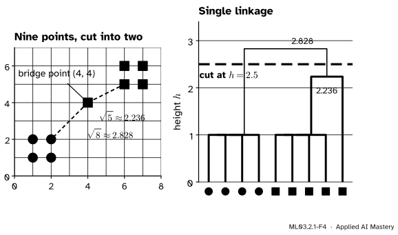
Now a two-dimensional case: the nine points of ML03.1, two squares of four and the bridge point \({(4, 4)}\). The two clusters that remain before the last merge are the two parts that the last merge joins.
nine = np.array([(1, 1), (2, 1), (1, 2), (2, 2), (6, 5), (7, 5), (6, 6), (7, 6), (4, 4)])merges9, _ = agglomerate_single(nine)print("heights:", np.round([h for _, _, h in merges9], 3))A, B, h = merges9[-1]print("last merge joins", nine[sorted(A)].tolist(), "and", nine[sorted(B)].tolist())
The nine points under single linkage. The bridge point is \({\sqrt{5} \approx 2.236}\) from the upper square and \({\sqrt{8} \approx 2.828}\) from the lower one, so it joins the upper square first. Cut between the two, the tree gives the same two clusters as k-means did in ML03.1.
Inside each square the nearest neighbours are 1 apart, so the first six merges all happen at \({h = 1}\). Then the bridge joins the upper square at \(\sqrt{5}\), and the two halves meet at \(\sqrt{8}\). The direct method scans every pair at every merge, about \({n^3/6}\) in all; the counter in the code confirms the 35 scans for six values. SciPy uses faster algorithms (ML03.2.4).
Explore
This module’s interactive, the dendrogram cutter, lives in lesson ML03.2.3. Load the six values or the nine points there, press Step to watch the merges happen one at a time, and compare the heights with the ones in this lesson.
Pitfalls
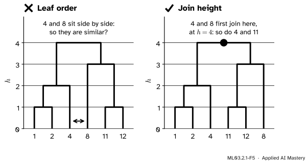
ML03.2.1-F5
Wrong beside right. Leaves that sit side by side need not be close: flipping any join gives an equally correct drawing with a different order. Only the height at which two leaves first join measures how far apart they are.
“Leaves next to each other in the dendrogram are similar.”
The left-to-right order is a drawing choice. At each of the \({n - 1}\) joins the two branches can be swapped without changing the tree, so there are \({2^{n-1}}\) correct drawings. In one drawing of the six values, 4 sits next to 8; in another it sits next to 11. In both, 4 first shares a cluster with either of them at \({h = 4}\). Read similarity from the height of the first common join.
“Hierarchical clustering finds the number of clusters for me.”
It postpones the choice; it does not make it. The tree holds every number of clusters from \(n\) to 1, and someone still has to cut it. Long vertical stretches with no joins hint at a natural cut, but that is a reading of the picture, not a result. Lesson ML03.2.3 treats cutting, and ML03.10 asks whether any clustering is really in the data.
“There are no iterations, so it must be cheap.”
There are no restarts and no convergence to wait for, but the direct method examines about \({n^3/6}\) distances and stores \({n(n - 1)/2}\) of them. That is fine for a few thousand points and hopeless for millions. For large data, single linkage has a much faster route (ML03.2.4), and the other linkages are usually run on a sample or with neighbourhood constraints.
Check yourself
Recall
1. In agglomerative clustering, what is a merge height?
Show answer
The distance between the two clusters at the moment they are merged, measured by the chosen linkage. It is the height at which the dendrogram draws that join.
2. How many merges does agglomerative clustering make on \(n\) points, and why?
Show answer
\({n - 1}\). It starts with \(n\) clusters, each merge removes one, and it stops when one is left.
3. How do you get \(K\) clusters from the dendrogram?
Show answer
Stop after \({n - K}\) merges, or equivalently cut the tree with a horizontal line between the \({(n - K)}\)-th and the \({(n - K + 1)}\)-th merge heights; each group of leaves still joined below the line is a cluster.
4. What is the single-linkage distance between two clusters?
Show answer
The distance between their closest pair of members, one from each cluster: \({D_{\min}(A, B) = \min d_{ij}}\) over \({i \in A}\) and \({j \in B}\).
5. What are the single-linkage merge heights of the values 1, 2, 4, 8, 11, 12?
Show answer
1, 1, 2, 3, 4.
Exercises
1.★ Run single linkage by hand on the values 0, 3, 4, 9, 10. Give the merges, their heights, and the two clusters left before the last merge.
Show solution
The gaps between neighbours are 3, 1, 5, 1, and single linkage on a line merges across these gaps from the smallest up. Merge \({\{3\} + \{4\}}\) at \({h = 1}\) and \({\{9\} + \{10\}}\) at \({h = 1}\) (a tie, either order). Next the smallest distance is \({D(\{0\}, \{3, 4\}) = 3}\), so merge at \({h = 3}\). Finally \({D(\{0, 3, 4\}, \{9, 10\})}\)\({= 9 - 4}\)\({= 5}\). Heights 1, 1, 3, 5; before the last merge the clusters are \({\{0, 3, 4\}}\) and \({\{9, 10\}}\).
2.★★ Show that for values on a line, single linkage merges across the gaps between neighbouring values in order of size, so its merge heights are those gaps sorted. Check it on the six values.
Show solution
Sort the values, \({x_{(1)} < \dots < x_{(n)}}\). Suppose every current cluster is a run of consecutive values; this is true at the start. For two runs \(R\) and \(S\) with \(R\) to the left of \(S\), the closest pair is the right end of \(R\) and the left end of \(S\). If a third run lies between them, it is closer to \(R\) than \(S\) is, so the smallest distance between clusters is always between two adjacent runs, and it equals the one gap that separates them. Merging two adjacent runs gives a run again, so the assumption holds at every step. Each merge therefore crosses one gap, always the smallest gap not yet crossed, and the heights are the \({n - 1}\) gaps in increasing order. For 1, 2, 4, 8, 11, 12 the gaps are 1, 2, 4, 3, 1, which sorted are 1, 1, 2, 3, 4.
3.★★★ Count the distances the direct method examines for \({n = 1{,}000}\) points, and estimate how much longer \({n = 10{,}000}\) takes. Then explain why SciPy’s single linkage, which needs only about \(n^2\) steps, still cannot handle \({n = 10^6}\) points on a laptop.
Show solution
\({(n^3 - n)/6}\) for \({n = 1{,}000}\) is \({166{,}666{,}500}\). Multiplying \(n\) by 10 multiplies \(n^3\) by 1,000, so \({n = 10{,}000}\) takes about a thousand times longer (about \({1.7 \times 10^{11}}\) comparisons). With an \(n^2\) algorithm the time grows only a hundredfold, but the input is still the \({n(n - 1)/2}\) distances: for \({n = 10^6}\) that is about \({5 \times 10^{11}}\) numbers, some 4 TB in double precision, far beyond a laptop’s memory.
Summary card
Merge the two closest clusters, again and again, and record each height.
ML03.2.1-F1
One tree holds every clustering.
Start:\(n\) clusters of one. Step: merge the pair with the smallest \({D(A, B)}\), record \(h\).
Single linkage: the distance of the closest pair; a merged cluster is as close to \(C\) as the closer of its two parts.
\(K\) clusters: stop after \({n - K}\) merges, or cut the tree between two heights.
Read heights, not leaf order. Cost of the direct method: \({(n^3 - n)/6}\) comparisons.
Sources and next steps
Sources. Each was opened and checked against this lesson on 15 November 2026.
G. James, D. Witten, T. Hastie and R. Tibshirani, An Introduction to Statistical Learning, 2nd edition (corrected printing, June 2023). Section 12.4.2: the dendrogram built from the leaves up, Algorithm 12.3 (fuse the two least dissimilar clusters, \({n - 1}\) times), a horizontal cut giving any number of clusters, and the warning that the \({2^{n-1}}\) reorderings of the leaves mean closeness along the horizontal axis says nothing.
T. Hastie, R. Tibshirani and J. Friedman, The Elements of Statistical Learning, 2nd edition, 12th printing. Section 14.3.12: agglomerative and divisive strategies, \({N - 1}\) levels in the hierarchy, the monotonicity property that lets a dendrogram be drawn, and single linkage (14.41).
SciPy developers, scipy.cluster.hierarchy.linkage: the \({(n-1) \times 4}\) matrix of merges, heights and cluster sizes, the single-linkage formula, and the note that all of its algorithms use memory of order \(n^2\).
Next.ML03.2.2 Linkage: what closest means replaces single linkage with complete, average and Ward linkage, and finds that the choice changes the tree.