Single, complete and average linkage measure the gap between two clusters by their closest, farthest or average pair, and Ward’s linkage by the rise in squared error. Derive Ward’s formula and the Lance-Williams update, and see the four trees of the six values.
ML03.2.2L2 Intermediate30 minIn review (what this means)
The maths and code on this page are checked by automated tests on every change, but an independent reader has not signed it off yet. Spot a mistake or a confusing step? Tell us.
Define single, complete and average linkage, and Ward’s linkage as the merge that raises the within-cluster sum of squares least.
Derive the rise in the within-cluster sum of squares when clusters A and B merge, n_A n_B / (n_A + n_B) times the squared distance between their means.
Use the Lance-Williams update to get every new distance from the old ones, and prove it for single and complete linkage.
Compute the merge heights of a small data set under all four linkages, including Ward’s heights in SciPy’s scale.
Predict when single linkage chains and when complete linkage gives compact groups.
The question
The last lesson merged “the two closest clusters” and quietly took closest to mean the closest pair of members. But a cluster is a set of points, and there are many fair ways to say how far apart two sets are. Which ways are there, do they change the tree, and which one should a data scientist pick?
From the last lesson
1. How many merges does agglomerative clustering make on \(n\) points?
Show answer
\({n - 1}\): it starts with \(n\) clusters, each merge removes one, and it stops at one.
2. What are the single-linkage merge heights of the values 1, 2, 4, 8, 11, 12?
Show answer
1, 1, 2, 3, 4.
Intuition
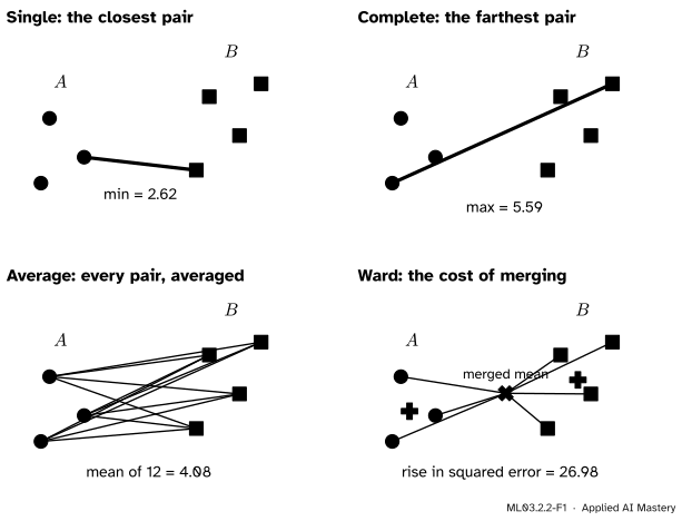
A linkage is a rule for the distance \({D(A, B)}\) between two clusters. Four rules cover almost all practice, and the picture shows each on the same pair of clusters.
ML03.2.2-F1
Four answers to “how far apart are \(A\) and \(B\)?”. Single linkage looks at one pair, complete linkage at the worst pair, average linkage at all of them, and Ward’s linkage at how much worse the clustering becomes if the two are merged.
Each rule has a character. Single linkage calls two clusters close if any one member of each is close, so it happily joins clusters through a thin line of points. Complete linkage calls them close only if every member of one is close to every member of the other, so it builds tight, round groups. Average linkage sits between the two. Ward’s linkage is the odd one out: it asks what the merge costs in the k-means objective, so it builds the kind of clusters k-means likes.
Build it up
Write \(n_A\) for the number of points in cluster \(A\) and \(d_{ij}\) for the distance between points \(i\) and \(j\).
Step 1. Single linkage: the closest pair.\({D_{\min}(A, B)}\) is the smallest \(d_{ij}\) with \(i \in A\) and \(j \in B\). One short distance is enough to make two clusters close.
Step 2. Complete linkage: the farthest pair.\({D_{\max}(A, B)}\) is the largest such \(d_{ij}\). A merge at height \(h\) guarantees that every pair inside the new cluster is at most \(h\) apart.
Step 3. Average linkage: every pair.\({D_{\text{avg}}(A, B)}\) is the mean of all \(n_A n_B\) distances between a member of \(A\) and a member of \(B\).
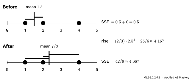
Step 4. Ward’s linkage: the cost of the merge. Recall the within-cluster sum of squares of ML03.1, the sum of squared distances from each point to the mean of its cluster. Merging two clusters can only raise it, because the merged points must share one mean. Ward’s rule merges the pair whose merge raises it least. On the six values, merging \({\{1, 2\}}\) with \(\{4\}\) costs:
ML03.2.2-F2
Ward’s cost of merging \({\{1, 2\}}\) and \(\{4\}\). Each bar is a distance to the cluster mean; the sum of squares adds their squares. It rises from 0.5 to \({42/9}\), by exactly \({25/6}\).
The rise, \({42/9 - 1/2 = 25/6}\), depends only on the sizes and the means: \({\tfrac{2 \cdot 1}{2 + 1} \cdot (4 - 1.5)^2}\)\({= \tfrac{2}{3} \cdot 6.25}\)\({= \tfrac{25}{6}}\). The next section proves that this always works.
The formal statement
NoteDefinition: four linkages
For clusters \(A\) and \(B\) with means \(\vect{\mu}_A\), \(\vect{\mu}_B\),
\({\Delta(A, B)}\) is the rise in the within-cluster sum of squares caused by merging \(A\) and \(B\).
Deriving Ward’s rise. Write \({S(C) = \sum_{i \in C} \norm{\vect{x}_i - \vect{\mu}_C}^2}\) for the sum of squares of a cluster \(C\). Expand the square and use \({\sum_{i \in C} \vect{x}_i = n_C \vect{\mu}_C}\):
The merged cluster has \({n_A + n_B}\) points, and its mean is the weighted mean of the two means, \({\vect{\mu} = (n_A \vect{\mu}_A + n_B \vect{\mu}_B)/(n_A + n_B)}\). In the rise \({\Delta = S(A \cup B) - S(A) - S(B)}\), the sums of \(\norm{\vect{x}_i}^2\) cancel, leaving
The middle step uses \({N n_A - n_A^2 = n_A n_B}\) and \({N n_B - n_B^2 = n_A n_B}\). Dividing by \(N\) gives the formula in the box. Two clusters with far-apart means are expensive to merge, and so are two large clusters: the factor \({n_A n_B / (n_A + n_B)}\) grows with both sizes.
SciPy’s scale for Ward. For two single points, \({\Delta = \tfrac{1}{2} d_{ij}^2}\). SciPy reports the Ward height \({h = \sqrt{2\Delta}}\), so that two single points merge at their distance, as under the other linkages. On the six values the rises are 1/2, 1/2, 25/6, 49/6 and 96, and the heights are 1, 1, 2.887, 4.041 and 13.856.
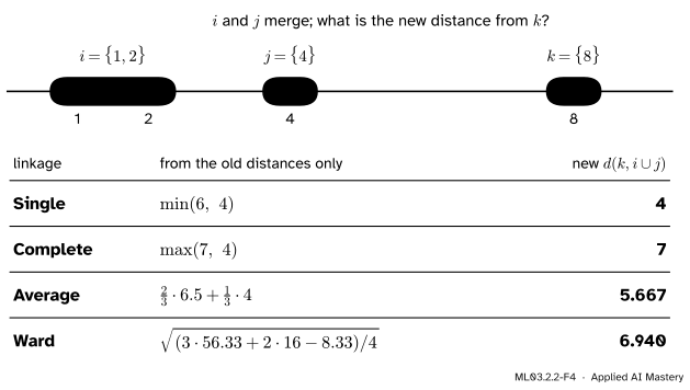
The Lance-Williams update. None of the four rules needs the original points once the merging has begun. When clusters \(i\) and \(j\) merge, the distance from any other cluster \(k\) to the new one is a fixed combination of three old distances:
(\(\alpha_j\) is \(\alpha_i\) with \(i\) and \(j\) swapped.) For single linkage, write \({a = d(k, i)}\) and \({b = d(k, j)}\). Then \({\tfrac12 a + \tfrac12 b - \tfrac12 \abs{a - b}}\) is \({\min(a, b)}\): if \({a \le b}\) it is \({\tfrac12 a + \tfrac12 b - \tfrac12 b + \tfrac12 a = a}\), and the other case is the same with the letters swapped. That is exactly the single-linkage update of ML03.2.1. With \({+\tfrac12}\) the same sum is \({\max(a, b)}\), which is complete linkage, because the farthest pair between \(k\) and \(i \cup j\) is the farther of the farthest pairs to \(i\) and to \(j\). For average linkage, the \({n_k(n_i + n_j)}\) pairs split into the \(n_k n_i\) pairs that reach \(i\) and the \(n_k n_j\) that reach \(j\), so the new mean is the size-weighted mean of the two old means. Ward’s row is stated here and checked in the code below.
ML03.2.2-F4
The Lance-Williams update at work on the six values. When \({\{1, 2\}}\) and \(\{4\}\) merge, the distance from \(\{8\}\) to the new cluster comes from the old distances alone, under every linkage.
Go deeper: a linkage whose heights can go down
Centroid linkage measures the distance between the two cluster means. Take three points at the corners of an equilateral triangle of side 1. Two of them merge at height 1, and their mean, the midpoint of one side, is only \({\sqrt{3}/2 \approx 0.866}\) from the third corner. So the second merge is lower than the first, an inversion, and the dendrogram’s joins cross. SciPy’s linkage offers "centroid" and gives heights 1 and 0.866 here.
Single, complete, average and Ward linkage never do this. Say \(i\) and \(j\) merge at the smallest current distance \(m\), so \({d(k, i) \ge m}\) and \({d(k, j) \ge m}\) for every other cluster \(k\). For the first three, the new distance is the minimum, the maximum or a weighted mean of those two, so it is at least \(m\). For Ward’s row (on squared heights, with \(m\) squared too), lowering \({d(k, i)}\) and \({d(k, j)}\) to \(m\) can only lower the result, and with all three old values equal to \(m\) it is exactly \(m\), because the three coefficients add up to \({(n_i + n_k) + (n_j + n_k) - n_k}\) over \(T\), which is 1. Either way no later merge can be lower.
Worked example
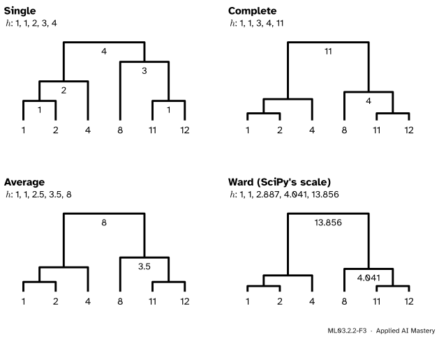
The six values under all four linkages. All four start the same way: \({\{1\} + \{2\}}\) and \({\{11\} + \{12\}}\) at height 1, the two smallest gaps. That leaves \({\{1, 2\}}\), \(\{4\}\), \(\{8\}\) and \({\{11, 12\}}\), and here the linkages part company. The three candidate merges are:
\({\{1, 2\}}\) with \(\{4\}\): single 2, complete 3, average 2.5, Ward \({\sqrt{25/3} \approx 2.887}\);
\(\{4\}\) with \(\{8\}\): 4 under all four (two single points);
\(\{8\}\) with \({\{11, 12\}}\): single 3, complete 4, average 3.5, Ward \({\sqrt{49/3} \approx 4.041}\).
Every linkage takes \({\{1, 2\} + \{4\}}\) next. Then the choice is between \({\{1, 2, 4\} + \{8\}}\) (single 4, complete 7, average \({17/3 \approx 5.667}\), Ward 6.940) and \({\{8\} + \{11, 12\}}\), which wins under every linkage. The last merge joins \({\{1, 2, 4\}}\) and \({\{8, 11, 12\}}\) at single 4, complete \({12 - 1 = 11}\), average 8 (the mean of the nine gaps across), and Ward \({\sqrt{2 \cdot 96} \approx 13.856}\), from the means \({7/3}\) and \({31/3}\), which are 8 apart: \({\tfrac{3 \cdot 3}{6} \cdot 8^2 = 96}\).
ML03.2.2-F3
The six values under the four linkages. Here the shape of the tree is the same every time and only the heights change; on less tidy data the shapes differ too.
Code
One function from scratch covers all four linkages through the Lance-Williams update. For Ward it works on squared heights and takes the square root at the end.
import numpy as npfrom scipy.cluster.hierarchy import linkagedef coefficients(method, ni, nj, nk):if method =="single":return0.5, 0.5, 0.0, -0.5if method =="complete":return0.5, 0.5, 0.0, 0.5if method =="average":return ni / (ni + nj), nj / (ni + nj), 0.0, 0.0 T = ni + nj + nk # Ward, on squared heightsreturn (ni + nk) / T, (nj + nk) / T, -nk / T, 0.0def agglomerate(X, method):"""Merge heights of agglomerative clustering, via the Lance-Williams update.""" X = np.asarray(X, dtype=float).reshape(len(X), -1) D = np.sqrt(((X[:, None, :] - X[None, :, :]) **2).sum(axis=2))if method =="ward": D = D **2 size = {i: 1for i inrange(len(X))} heights = []whilelen(size) >1: live =sorted(size) best =min((D[i, j], i, j) for i in live for j in live if i < j) h, i, j = best heights.append(np.sqrt(h) if method =="ward"else h)for k in live:if k in (i, j):continue ai, aj, b, g = coefficients(method, size[i], size[j], size[k]) D[k, i] = D[i, k] = (ai * D[k, i] + aj * D[k, j] + b * D[i, j]+ g *abs(D[k, i] - D[k, j])) size[i] += size.pop(j)return np.array(heights)values = np.array([1, 2, 4, 8, 11, 12])for method in ["single", "complete", "average", "ward"]: ours = agglomerate(values, method) scipy_heights = linkage(values.reshape(-1, 1), method)[:, 2]print(f"{method:9s}", np.round(ours, 3), " SciPy agrees:", np.allclose(ours, scipy_heights))
Ward’s heights in SciPy’s scale are \(\sqrt{2\Delta}\). Recovering the rises in the within-cluster sum of squares, and checking them against a direct computation:
rises from SciPy: [ 0.5     0.5     4.1667  8.1667 96.    ]
rises by hand:    [ 0.5     0.5     4.1667  8.1667 96.    ]
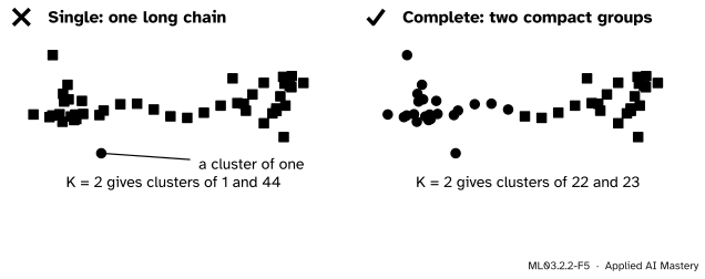
Now the character of single and complete linkage, on 45 seeded points: two round blobs of 18 joined by a chain of 9. Cut each tree into two clusters and count.
single    cluster sizes: [1, 44]
complete  cluster sizes: [22, 23]
average   cluster sizes: [21, 24]
ward      cluster sizes: [19, 26]
fcluster with criterion="maxclust" cuts a tree into at most the given number of clusters; lesson ML03.2.3 explains it. Single linkage walks along the chain and joins everything, leaving one stray point as the second “cluster”. Complete linkage splits the data into two compact halves.
Explore
The dendrogram cutter in lesson ML03.2.3 switches between the four linkages on the same points. Load the six values and watch the heights change while the shape stays; then drag one point into the gap between the groups and see single linkage start to chain.
Pitfalls
ML03.2.2-F5
Wrong beside right, both cut into two clusters. Single linkage joins the blobs through the chain and the “second cluster” is one stray point. Complete linkage gives two compact groups.
“Single linkage is the natural meaning of closest, so it is the safe default.”
Single linkage needs only one short distance to join two clusters, so a chain of points, or a single bridge point, glues groups together; ESL calls this chaining. Its clusters can be long and thin, with members far apart. It is useful when clusters really are long and thin, and it is fast (ML03.2.4), but for compact groups prefer complete, average or Ward linkage. scikit-learn’s AgglomerativeClustering uses Ward by default.
“Ward heights are distances, comparable with the other linkages.”
Ward’s natural number is the rise \(\Delta\) in the sum of squares. SciPy and scikit-learn report \(\sqrt{2\Delta}\), which equals the distance only for two single points. For larger clusters it grows with the cluster sizes: the final Ward height of the six values is 13.856, larger than any distance in the data (the largest is 11). Compare heights within one tree, not across linkages.
“Any linkage works with any distance.”
Single, complete and average linkage use the distances alone, so they work with any dissimilarity, including ones that are not Euclidean. Ward’s rule is built on means and squared Euclidean distance; SciPy states that "ward" is correctly defined only for Euclidean distances, and scikit-learn accepts only the Euclidean metric with it. For other distances, average linkage is the usual choice.
Check yourself
Recall
1. Define complete linkage, and say what a complete-linkage merge at height \(h\) guarantees.
Show answer
\({D_{\max}(A, B)}\) is the largest distance between a member of \(A\) and a member of \(B\). A merge at height \(h\) guarantees that every pair of points in the merged cluster is at most \(h\) apart.
2. What does Ward’s linkage minimise at each merge?
Show answer
The rise in the within-cluster sum of squares, \({\Delta = \tfrac{n_A n_B}{n_A + n_B} \norm{\vect{\mu}_A - \vect{\mu}_B}^2}\).
3. In which scale does SciPy report Ward heights?
Show answer
\({h = \sqrt{2\Delta}}\), so that two single points merge at their distance.
4. Which Lance-Williams coefficients give single linkage, and why?
Show answer
\({\alpha_i = \alpha_j = \tfrac12}\), \({\beta = 0}\), \({\gamma = -\tfrac12}\), because \({\tfrac12 a + \tfrac12 b - \tfrac12 \abs{a - b}}\)\({= \min(a, b)}\).
5. What is chaining?
Show answer
Single linkage joining two groups through a series of close intermediate points, so that a cluster becomes long and thin and its members can be far apart.
Exercises
1.★ Clusters \({A = \{0, 2\}}\) and \({B = \{5, 9\}}\) lie on a line. Compute their single, complete and average linkage distances, and Ward’s rise \(\Delta\).
Show solution
The four cross distances are 5, 9, 3 and 7. Single: 3. Complete: 9. Average: \({(5 + 9 + 3 + 7)/4 = 6}\). Ward: the means are 1 and 7, so \({\Delta = \tfrac{2 \cdot 2}{4} \cdot 6^2 = 36}\). Check directly: \({S(A) = 2}\), \({S(B) = 8}\), and the merged mean is 4, so \({S(A \cup B) = 16 + 4 + 1 + 25 = 46}\), and \({46 - 2 - 8 = 36}\).
2.★★ Check Ward’s Lance-Williams row on the six values. With \({i = \{1, 2\}}\), \({j = \{4\}}\), \({k = \{8\}}\), find the three old squared heights \({h^2 = 2\Delta}\), apply the update and compare with \(\Delta\) computed directly for \({\{1, 2, 4\}}\) and \(\{8\}\).
Show solution
The old squared heights are \({h^2(k, i) = 2 \cdot \tfrac{2 \cdot 1}{3} \cdot 6.5^2}\)\({= \tfrac{169}{3}}\)\({\approx 56.33}\), \({h^2(k, j) = 4^2 = 16}\) and \({h^2(i, j) = 2 \cdot \tfrac{25}{6} = \tfrac{25}{3}}\). With \({n_i = 2}\), \({n_j = n_k = 1}\) and \({T = 4}\), the update gives
Directly: the means are \({7/3}\) and 8, so \({\Delta = \tfrac{3 \cdot 1}{4} \cdot (17/3)^2 = \tfrac{289}{12}}\) and \({2\Delta = \tfrac{578}{12}}\). They agree, and the height is \({\sqrt{48.17} \approx 6.940}\).
3.★★★ ESL notes that single and complete linkage depend only on the order of the distances, while average linkage does not. Show that replacing every \(d_{ij}\) by \(d_{ij}^2\) never changes the single-linkage merges, then run average linkage on the values 0, 7, 15, 27 with plain and with squared distances and compare the two clusters left before the last merge.
Show solution
Squaring is increasing on non-negative numbers, so it keeps the order of the distances, and the minimum of squares is the square of the minimum. Every comparison single linkage makes, and so every merge, is unchanged; only the heights are squared.
Average linkage, plain distances. The smallest gap is 7, so \({\{0\} + \{7\}}\) first. Then \({D(\{0, 7\}, \{15\})}\)\({= (15 + 8)/2}\)\({= 11.5}\) and \({D(\{15\}, \{27\}) = 12}\), so \(\{15\}\) joins \({\{0, 7\}}\). The two clusters are \({\{0, 7, 15\}}\) and \(\{27\}\).
Squared distances. The first merge is again \({\{0\} + \{7\}}\), at 49. Then \({D(\{0, 7\}, \{15\})}\)\({= (225 + 64)/2}\)\({= 144.5}\) but \({D(\{15\}, \{27\}) = 144}\), so now \(\{15\}\) joins \(\{27\}\). The two clusters are \({\{0, 7\}}\) and \({\{15, 27\}}\). A mean of distances is not preserved by an increasing transformation, so average linkage can change its merges; a minimum or a maximum is preserved, so single and complete linkage cannot.
Summary card
A linkage says how far apart two clusters are; each one builds a different kind of cluster.
ML03.2.2-F1
Closest, farthest, average, cost.
Single \(\min d_{ij}\) (chains), complete \(\max d_{ij}\) (compact), average: mean of \(n_A n_B\) pairs.
Lance-Williams: \({d(k, i \cup j)}\) from \({d(k, i)}\), \({d(k, j)}\), \({d(i, j)}\) alone.
Six values: complete 1, 1, 3, 4, 11; average 1, 1, 2.5, 3.5, 8; Ward 1, 1, 2.887, 4.041, 13.856.
Sources and next steps
Sources. Each was opened and checked against this lesson on 15 November 2026.
T. Hastie, R. Tibshirani and J. Friedman, The Elements of Statistical Learning, 2nd edition, 12th printing. Section 14.3.12: single (14.41), complete (14.42) and group average (14.43) linkage; chaining and the large diameters of single-linkage clusters; complete linkage’s compact clusters; and the invariance of single and complete linkage, but not group average, under monotone transformations of the dissimilarities.
G. James, D. Witten, T. Hastie and R. Tibshirani, An Introduction to Statistical Learning, 2nd edition. Section 12.4.2 and Table 12.3: complete, average, single and centroid linkage, and the inversions that centroid linkage can produce.
SciPy developers, scipy.cluster.hierarchy.linkage: the formulas for each method, including the Ward update on squared distances with \({T = \abs{v} + \abs{s} + \abs{t}}\), and the statement that centroid, median and Ward are correctly defined only for Euclidean distances.
scikit-learn developers, User Guide, Section 2.3.6: Hierarchical clustering (version 1.9): the four linkage criteria, Ward as a variance-minimising approach like the k-means objective, single linkage as the most brittle and the cheapest to compute, and average linkage as the alternative for non-Euclidean metrics.