Prove that EM never lowers the likelihood: Jensen’s inequality gives a lower bound that the E-step makes touch and the M-step raises. Then find k-means as EM’s hard limit, and meet the collapse and the local optima that the proof does not rule out.
ML03.4.3L2 Intermediate25 minIn review (what this means)
The maths and code on this page are checked by automated tests on every change, but an independent reader has not signed it off yet. Spot a mistake or a confusing step? Tell us.
State Jensen’s inequality for the logarithm and use it to build a lower bound on the log-likelihood for any distribution over the latent labels.
Prove that the E-step makes the bound touch the log-likelihood and the M-step raises it, so the log-likelihood never decreases.
Derive k-means as the limit of EM for a mixture whose shared variance shrinks to zero.
Explain the collapse of a component onto one point and the local optima of EM, and apply the remedies: a variance floor, several starts and k-means initialisation.
The question
On the six values the log-likelihood went \(-14.429\), \(-13.258\), \(-12.764\), \(-12.726\): up every time. Is that luck, or a law? And if it is a law, why did three components on the same six values end with a much higher log-likelihood and a worse model?
From the last lesson
1. Write the M-step update for the mean of component \(k\).
Show answer
\({\mu_k = \sum_i r_{ik} x_i / N_k}\) with \({N_k = \sum_i r_{ik}}\): the responsibility-weighted mean.
2. What does the M-step maximise?
Show answer
The responsibility-weighted log-likelihood, with the responsibilities from the E-step held fixed:
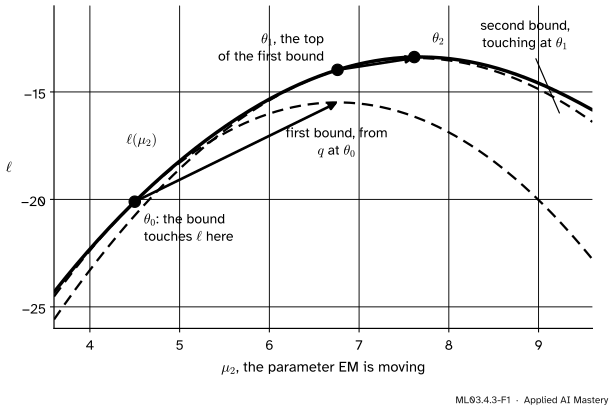
EM climbs a hill it cannot see whole. At the current parameters \(\theta_t\), the E-step builds a simpler curve that lies everywhere below the log-likelihood and touches it at \(\theta_t\). The M-step jumps to the top of that simpler curve. The log-likelihood there is at least as high as the curve, which is at least as high as where we started. Then a new curve is built at the new point.
ML03.4.3-F1
EM on a one-parameter slice of the six-value problem. Each dashed curve is a lower bound that touches \(\ell\) at the current value. Jumping to the bound’s top (green) lands under a higher point of \(\ell\), so every step goes up.
The whole proof is in this picture. What needs showing is that the dashed curves exist: that the E-step really produces a bound that touches, and that maximising it is the M-step of the last lesson.
Build it up
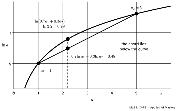
Step 1. The logarithm bends down. Take two positive numbers \({a_1 = 1}\) and \({a_2 = 5}\) and weights \({0.7}\) and \({0.3}\). The log of their weighted average is \({\ln 2.2 = 0.79}\); the weighted average of their logs is \({0.3 \ln 5 = 0.48}\). The first is larger, because the chord between two points of a curve that bends down lies below the curve.
ML03.4.3-F2
Jensen’s inequality for the logarithm. The log of an average (green) is never below the average of the logs (vermillion), because the logarithm curves downwards.
Step 2. Jensen’s inequality. For weights \({q_k \ge 0}\) that add to 1 and positive numbers \(a_k\),
with equality exactly when all the \(a_k\) with \({q_k > 0}\) are equal. (Bishop proves the general form for any curve that bends one way, in his section 1.6.1.)
Step 3. Make the log-likelihood look like the left side. Each term of \(\ell\) is the log of a sum, \({\ln \sum_k \pi_k N_{ik}}\), where \({N_{ik} = N(x_i \mid \mu_k, \sigma_k^2)}\). It is not yet a weighted average. Make it one: pick any weights \(q_{ik}\) for point \(i\), and multiply and divide each term by its weight.
The formal statement
NoteTheorem: the lower bound, and why EM climbs
For any parameters \(\theta\) and any weights \({q_{ik} > 0}\) with \({\sum_k q_{ik} = 1}\) for each point,
with equality when \({q_{ik} = r_{ik}(\theta)}\), the responsibilities. Hence each EM iteration gives \({\ell(\theta_{t+1}) \ge \ell(\theta_t)}\).
Proof of the bound. For one point, multiply and divide by \(q_{ik}\), then use Jensen with weights \(q_{ik}\) and numbers \({a_k = \pi_k N_{ik} / q_{ik}}\):
where \({Q(\theta) = \sum_{i,k} q_{ik} \ln(\pi_k N_{ik})}\). With \(q\) fixed the second sum is a constant, so maximising \(L\) over \(\theta\) is maximising \(Q\): exactly the M-step of the last lesson.
The climb. Let \(q_{t+1}\) be the responsibilities at \(\theta_t\) and \(\theta_{t+1}\) the M-step’s answer.
Each inner sum is the Kullback-Leibler divergence from the distribution \(q_i\) to the responsibilities \(r_i(\theta)\), a measure of how far apart two distributions are (M09.3 treats it in full). By Jensen it is never negative, and it is zero only when \({q_i = r_i}\). This is Bishop’s decomposition (9.70). The general theory, for any model with hidden variables, is ML05.7, and the bound reappears as the ELBO of variational inference in M09.8.
k-means is EM’s hard limit. Give every component the same variance \(\varepsilon\), held fixed, and fixed positive weights. In \(d\) dimensions the constants \({(2\pi\varepsilon)^{-d/2}}\) cancel from the responsibilities, leaving, with \({d_{ik} = \norm{\vect{x}_i - \vect{\mu}_k}}\),
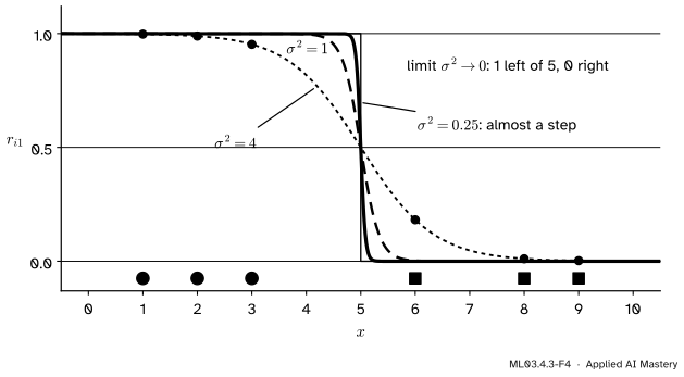
If the nearest centre is unique, each \({d_{ij}^2 - d_{ik^*}^2}\) is positive, so as \({\varepsilon \to 0}\) every exponential goes to 0 and \({r_{ik^*} \to 1}\). The E-step becomes “give each point wholly to its nearest centre”, and the M-step for the means becomes “move each centre to the mean of its points”. That is Lloyd’s algorithm. Moreover \(Q\) is \({-\tfrac{1}{2\varepsilon}\sum_{i,k} r_{ik} d_{ik}^2}\) plus terms that do not involve the means, so maximising \(Q\) is minimising the k-means objective \(J\).
ML03.4.3-F4
Responsibilities for components at 2 and 8 with a shared variance, \({r_{i1} = \sigma(6(5 - x)/\sigma^2)}\). As the variance shrinks the curve steepens into a step at 5: every point goes wholly to the nearer centre, as in k-means.
Worked example
Check the sandwich on the six values, and look inside it at the value 6.
From the start \(\theta_0\), the E-step gives \({q = r(\theta_0)}\); for the value 6 that is \({(0.1824, 0.8176)}\). Both ratios \({\pi_k N_{ik} / q_{ik}}\) equal \({p(6) = 0.07399}\): \({0.01350 / 0.1824 = 0.07399}\) and \({0.06049 / 0.8176 = 0.07399}\). So the point’s share of the bound is \({\ln 0.07399 = -2.604}\), exactly \({\ln p(6)}\). The bound touches.
Now keep that \(q\) and move to the M-step’s \(\theta_1\). The weighted components at 6 are now 0.00230 and 0.06713, so the ratios are \({0.00230 / 0.1824 = 0.0126}\) and \({0.06713 / 0.8176 = 0.0821}\), no longer equal. The point’s share of the bound is
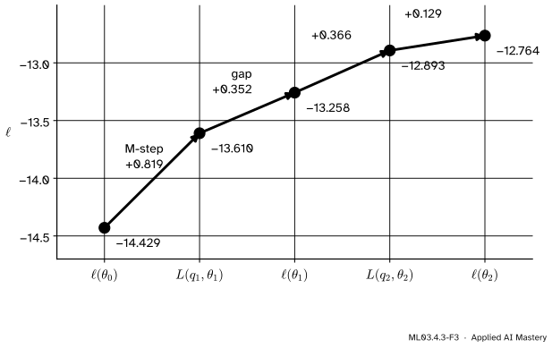
below the true \({\ln p_{\theta_1}(6) = \ln 0.06944 = -2.667}\). For this one point the bound even went down: the M-step raises the total, not every term. Added over all six points:
ML03.4.3-F3
The worked-example trace. Each M-step raises the bound (green); the gap between bound and log-likelihood adds more (reddish purple). Every arrow points up.
The first iteration reads \({-14.429 = L(q_1, \theta_0)}\), then \({L(q_1, \theta_1) = -13.610}\), then \({\ell(\theta_1) = -13.258}\). The M-step gained 0.819 and the gap added 0.352. The second iteration goes \(-13.258\), \(-12.893\), \(-12.764\). Both inequalities hold at every step.
Code
From scratch: compute the bound and check the sandwich over thirty iterations.
The k-means limit, on the nine points of ML03.1 started from the centres \((1, 1)\) and \((2, 1)\): EM with a fixed shared variance of 0.01 and equal weights moves the centres exactly as Lloyd’s algorithm does.
\(J\) falls 179, 23.918, 10.8, and every responsibility is 0 or 1 to machine precision. Now the collapse: place component 1 on the value 1 and shrink its variance, while component 2 covers the other five values.
The library’s defences: reg_covar adds a small number to every variance, n_init runs several starts and keeps the best, and init_params='kmeans' (the default) starts from a k-means answer. On four blobs, thirty runs from random data points end at different heights:
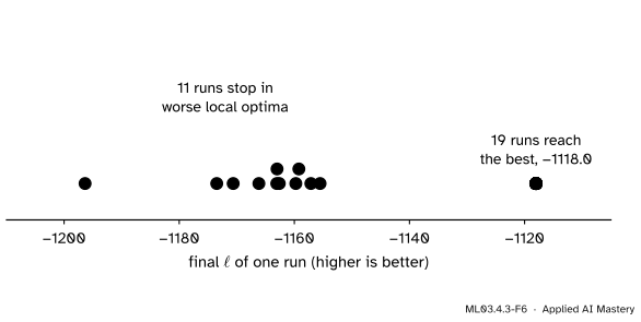
About a third of the random starts stop at least 30 below the best value, near \(-1118\); ten starts, or one k-means start, find the best.
Explore
The EM stepper in lesson ML03.4.2 traces \(\ell\) after every M-step: the trace never goes down. With three components on the six values, watch one component shrink onto the single value 6 until the stepper’s variance floor holds it: the collapse of this lesson. With the tilted blobs and Random start, compare the final values.
Pitfalls
ML03.4.3-F5
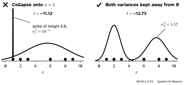
Wrong beside right. A component that sits on one point and shrinks its variance scores a higher log-likelihood (\(-11.12\), and rising without limit) than the honest fit (\(-12.73\)), while describing the data worse.
“A higher log-likelihood always means a better fit.”
Not for mixtures. Put one component’s mean on a data point and let its variance shrink: that point’s density grows like \({1/\sqrt{2\pi\sigma^2}}\), without limit, while the other component keeps the rest finite. So \(\ell\) has no maximum at all; it goes to infinity. EM can walk into this collapse. A floor on the variances (reg_covar) and several starts keep it in a sensible local maximum.
ML03.4.3-F6
Thirty EM runs from random starts on four blobs. Most reach the same best value; the rest stop lower, in local optima where one component straddles two blobs while the spare one splits a blob or holds a few stray points.
“EM converged, so it found the maximum-likelihood fit.”
The proof says only that \(\ell\) never falls. EM stops wherever the bound’s top is its touching point, which can be a local maximum far below the best. Run several starts (n_init) and keep the highest, or start from k-means.
“Starting every component at the same place is a neutral start.”
It is a trap. If all components start identical, every point gives them equal responsibilities, so the M-step moves them identically, for ever. On the six values two identical components settle on mean 4.833 and variance 9.139: one Gaussian, with \({\ell = -15.151}\). Break the symmetry at the start.
Check yourself
Recall
1. State Jensen’s inequality for the logarithm.
Show answer
For weights \({q_k \ge 0}\) adding to 1 and positive \(a_k\), \({\ln \sum_k q_k a_k \ge \sum_k q_k \ln a_k}\), with equality when all the \(a_k\) are equal.
2. For which choice of \(q\) does the lower bound touch the log-likelihood?
Show answer
When \({q_{ik} = r_{ik}}\), the responsibilities at the current parameters. Then every ratio \({\pi_k N_{ik} / q_{ik}}\) equals \(p(x_i)\).
3. Write the two inequalities that show \({\ell(\theta_{t+1}) \ge \ell(\theta_t)}\).
Show answer
The E-step makes the bound touch, the M-step maximises it, and the bound lies below \(\ell\):
All components share one fixed variance \(\varepsilon\), and \({\varepsilon \to 0}\). The responsibilities become 0 or 1 for the nearest centre, and the mean update becomes the k-means update.
5. Name three remedies for collapse and local optima.
Show answer
A floor on the variances (reg_covar), several starts keeping the best (n_init), and starting from k-means (init_params='kmeans').
Exercises
1.★ For components at 2 and 8 with equal weights and a shared variance \(\varepsilon\), show that \({r_{i1} = \sigma(6(5 - x)/\varepsilon)}\), and find \(r_{i1}\) for \({x = 6}\) when \({\varepsilon = 1}\).
Show solution
As in ML03.4.1, \({r_{i1} = \sigma(a)}\) with \({a = ((x - 8)^2 - (x - 2)^2)/(2\varepsilon)}\). The numerator is \({60 - 12x = 12(5 - x)}\), so \({a = 6(5 - x)/\varepsilon}\). For \({x = 6}\) and \({\varepsilon = 1}\), \({a = -6}\) and \({r_{i1} = 1/(1 + e^{6}) = 0.0025}\).
2.★★ In the collapse, component 1 has weight \(\tfrac16\), mean 1 and variance \(s\). Show that the term of \(\ell\) for the value 1 is at least \({\ln \tfrac16 - \tfrac12 \ln(2\pi s)}\), and find how small \(s\) must be for that alone to exceed 0.
Show solution
\({p(1) \ge \tfrac16 N(1 \mid 1, s) = \tfrac16 (2\pi s)^{-1/2}}\), because the other term is positive. Take logs. The bound exceeds 0 when \({(2\pi s)^{-1/2} > 6}\), that is \({s < 1/(72\pi) = 0.0044}\). Below that, one point contributes a positive amount, and the total grows without limit as \({s \to 0}\).
3.★★★ Show that the M-step raises the bound even though, for the value 6 in the worked example, that point’s share of the bound fell from \(-2.604\) to \(-2.841\). Where did the gain come from?
Show solution
The M-step maximises the sum\({L(q_1, \theta) = \sum_i L_i}\) over \(\theta\), and the start \(\theta_0\) is one of the candidates, so the maximum is at least \({L(q_1, \theta_0)}\). Individual terms may fall. Here the variances shrank from 4 to about 1.66 and 1.97, which raises the density, and so the share, of the points near the means. The shares of 1, 2, 3 and 8 rise (for 2, from \(-2.294\) to \(-1.870\)); those of 6 and 9 fall. The gains are larger, and the total rises from \(-14.429\) to \(-13.610\).
Summary card
EM touches \(\ell\) from below, then climbs the bound.
ML03.4.3-F1
Touch, climb, repeat.
Bound.\({\ell(\theta) \ge \sum_{i,k} q_{ik} \ln(\pi_k N_{ik} / q_{ik})}\), by Jensen.
E-step.\({q = r(\theta_t)}\) makes it touch.
M-step. Maximise the bound, so \({\ell(\theta_{t+1}) \ge \ell(\theta_t)}\).
Limits. Shared variance \({\to 0}\) gives k-means; a variance \({\to 0}\) on one point gives \({\ell \to \infty}\).
Sources and next steps
Sources. Each was opened and checked against this lesson on 15 November 2026.
Christopher M. Bishop, Pattern Recognition and Machine Learning, Springer 2006. Section 1.6.1: Jensen’s inequality (1.115). Section 9.2.1: the singularity (9.15), where a component “collapses” onto a data point and the log-likelihood goes to infinity. Section 9.3.2: k-means as the limit \({\varepsilon \to 0}\) of a mixture with covariances \({\varepsilon \mat{I}}\), responsibilities (9.42) and the expected complete-data log-likelihood (9.43). Section 9.4: the decomposition \({\ln p = L(q, \theta) + \mathrm{KL}(q \,\|\, p)}\) (9.70) to (9.72), and the E-step and M-step as raising the bound (Figures 9.12 to 9.14).
T. Hastie, R. Tibshirani and J. Friedman, The Elements of Statistical Learning, 2nd edition, corrected 12th printing (2017). Section 8.5.1: the spike of infinite height at a data point and several starting guesses. Section 8.5.2: the proof that EM “never decreases the log-likelihood” (8.47). Section 8.5.3: EM as maximisation over both arguments of one function (8.48). Section 14.3.7: Gaussian mixtures as soft k-means, with hard assignments as \({\sigma^2 \to 0}\).
scikit-learn, sklearn.mixture.GaussianMixture (version 1.9.1): reg_covar (default \(10^{-6}\)), n_init (default 1) and init_params (default 'kmeans', or 'k-means++', 'random', 'random_from_data'); and the User Guide, section 2.1, on singularities and “solutions with infinite likelihood unless one regularizes the covariances artificially”.
Next.ML03.4.4 Gaussian mixtures in the plane gives each component a covariance matrix, fits the tilted clusters that k-means cut the wrong way, and uses BIC to choose how many components to keep.