PCA cannot unroll a rolled-up sheet, because it trusts every straight-line distance. Join each point to its nearest neighbours only, and the bottom eigenvectors of the graph Laplacian lay the sheet out flat: Laplacian eigenmaps, spectral clustering and Isomap.
ML03.6.1L2 Intermediate30 minIn review (what this means)
The maths and code on this page are checked by automated tests on every change, but an independent reader has not signed it off yet. Spot a mistake or a confusing step? Tell us.
Build a k-nearest-neighbour graph with Gaussian edge weights and its Laplacian L = D - W.
Derive that minimising the weighted sum of squared embedded distances, under a scale constraint, gives the generalised eigenproblem L y = lambda D y.
Compute a Laplacian eigenmap by hand on four points and from scratch on make_swiss_roll, and match it with SpectralEmbedding.
Cluster make_moons and make_circles by k-means on a spectral embedding, and explain the short circuit that a large k causes.
The question
Roll a sheet of paper into a tube and scatter 800 dots on it. Two dots on neighbouring turns of the roll can be closer through the air than two dots far apart on the same turn. PCA (ML03.5) only sees straight-line distances, so it cannot tell them apart. How can a method flatten the sheet when the only distances it can trust are the short ones?
Intuition
The idea is to stop trusting long distances. Over a short range a curved sheet looks flat, so a point’s nearest neighbours really are its neighbours on the sheet. Join each point to those few neighbours and nothing else, and the result is a neighbourhood graph: a net that follows the sheet and never jumps across the gap between two turns.
ML03.6.1-F1
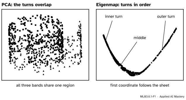
The swiss roll, cut into three bands along the sheet. Left: PCA’s best flat view lays the turns on top of each other. Right: a Laplacian eigenmap of the 10-nearest-neighbour graph keeps the bands in their order along the sheet.
Now ask for positions on a line, or in the plane, that keep every joined pair close. Pairs that are not joined are free to end up far apart. That one request, pull neighbours together and ignore everyone else, is what unrolls the sheet. Its answer turns out to be an eigenvector problem, the same graph Laplacian that cut a graph in two in M03.9.3.
Build it up
Step 1. The data.make_swiss_roll draws points \(\cdata{\vect{x}_i}\) in \(\R^3\) on a rectangle rolled into a spiral. Its second output, \(t\), is each point’s position along the sheet, from about 4.7 to 14.1. The method never sees \(t\); we keep it to check the answer.
Step 2. The graph. Join \(i\) and \(j\) if either is among the other’s \(k\) nearest neighbours. This k-nearest-neighbour graph is symmetric by construction.
Step 3. The weights. Give each edge a Gaussian weight, close to 1 for a short edge and smaller for a long one, and put \(w_{ij} = 0\) where there is no edge:
The bandwidth \(\cparam{\sigma}\) sets what counts as short. A common choice, used here, is the median distance from a point to its \(k\) nearest neighbours.
ML03.6.1-F2
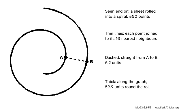
The roll seen end on, with its 10-nearest-neighbour graph. A and B are 6.2 apart in a straight line, but the graph has no edge across the gap, so its shortest path between them runs 59.9 units round the sheet.
Step 4. The cost. Give each point a coordinate \(\cmodel{y_i}\) on a line and add up a spring energy, one term per edge:
A heavy edge whose ends are far apart costs a lot. A pair with no edge costs nothing, however far apart it lands. The best layout is the one with the smallest \(\closs{E}\).
Step 5. Two guards. Putting every \(y_i\) equal makes \(\closs{E} = 0\) and tells us nothing. So we fix the scale and forbid the constant answer; the next section turns these guards into equations.
The formal statement
Write \(\mat{W}\) for the matrix of weights, \(\mat{D}\) for the diagonal matrix of degrees\({d_i = \sum_j w_{ij}}\), and \(\mat{L} = \mat{D} - \mat{W}\) for the graph Laplacian of M03.9.3.
The cost is a quadratic form. Expand \({(y_i - y_j)^2 = y_i^2 - 2y_iy_j + y_j^2}\) and use \({w_{ij} = w_{ji}}\):
The third line sums \(w_{ij}\) over \(j\) to get \(d_i\) in the first term, and over \(i\) to get \(d_j\) in the last. Since \(\closs{E} \ge 0\) for every \(\vect{y}\), \(\mat{L}\) is positive semidefinite.
NoteResult: the Laplacian eigenmap (Belkin and Niyogi)
Minimise \({\vect{y}\T\mat{L}\vect{y}}\) subject to \({\vect{y}\T\mat{D}\vect{y} = 1}\) and \({\vect{y}\T\mat{D}\vect{1} = 0}\). The minimiser solves the generalised eigenproblem
\[
\mat{L}\vect{y} = \lambda\,\mat{D}\vect{y}
\]
for the smallest eigenvalue after \(\lambda_0 = 0\). For a map into \(\R^q\), use the eigenvectors of the \(q\) smallest eigenvalues after 0 as the \(q\) coordinates.
Derivation. The first guard fixes the scale; \(\mat{D}\) in it gives well-connected points more say. Bring it in with a Lagrange multiplier \(\lambda\) and set the gradient to zero:
So \(\vect{y}\) must be a generalised eigenvector. Multiply \({\mat{L}\vect{y} = \lambda\mat{D}\vect{y}}\) on the left by \(\vect{y}\T\): the cost is \({\vect{y}\T\mat{L}\vect{y} = \lambda\,\vect{y}\T\mat{D}\vect{y} = \lambda}\), so the smallest cost belongs to the smallest eigenvalue. That is \(\lambda_0 = 0\), with \(\vect{y} = \vect{1}\), because every row of \(\mat{L}\) sums to zero. The second guard forbids it, so the answer is the next eigenvector. That one meets the second guard by itself: if \({\mat{L}\vect{y}_a = \lambda_a\mat{D}\vect{y}_a}\) and \({\mat{L}\vect{y}_b = \lambda_b\mat{D}\vect{y}_b}\), then \({\vect{y}_b\T\mat{L}\vect{y}_a}\) equals both \({\lambda_a\,\vect{y}_b\T\mat{D}\vect{y}_a}\) and \({\lambda_b\,\vect{y}_b\T\mat{D}\vect{y}_a}\), so \({\vect{y}_b\T\mat{D}\vect{y}_a = 0}\) whenever \({\lambda_a \ne \lambda_b}\). On a connected graph the constant is the only eigenvector with \(\lambda = 0\), so the next one has \(\lambda_1 > 0\).
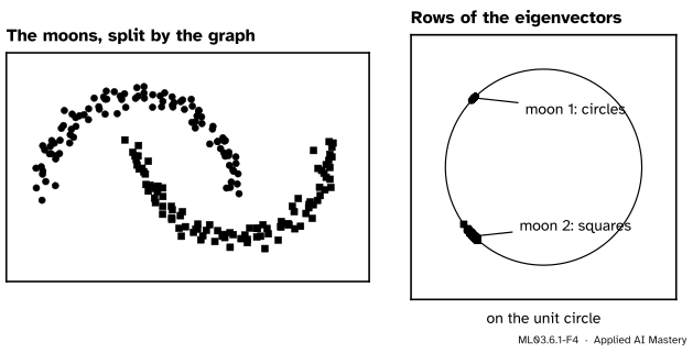
Spectral clustering uses the same eigenvectors for grouping (Ng, Jordan and Weiss, 2001). Take the \(K\) smallest eigenvectors of the normalised Laplacian \({\mat{I} - \mat{D}^{-1/2}\mat{W}\mat{D}^{-1/2}}\), stack them as columns, rescale each row to length 1, and run k-means (ML03.1) on the rows. Points that the graph joins get nearly equal rows, so clusters of any shape become round, tight groups.
ML03.6.1-F4
Spectral clustering of make_moons. Right: each point’s row of the two smallest eigenvectors, rescaled to length 1. Each moon collapses to almost one spot on the circle, and k-means separates the two spots at once. Left: those labels back on the data.
Go deeper: Isomap: unroll by measuring along the graph
Isomap uses the same graph differently. It weights each edge by its length, takes the shortest path through the graph between every pair of points (the 59.9 of the figure above, not the straight 6.2), and hands that matrix of distances to classical multidimensional scaling (ML03.5.2): double-centre the squared distances and keep the top eigenvectors. Where the eigenmap only keeps neighbours together, Isomap tries to keep every along-the-sheet distance, so on the swiss roll it returns a flat rectangle. The code below builds it with scipy.sparse.csgraph.shortest_path and matches sklearn.manifold.Isomap.
Worked example
Lay four points round a bend on a line. Take \(A = (0, 0)\), \(B = (1, 0)\), \(C = (1.5, 0.866)\) and \(D = (1, 1.732)\): three steps of length 1, each turning by 60°. The other distances are \({AC = BD = \sqrt{3}}\) and \({AD = 2}\).
The graph, with \(k = 2\).\(A\)’s two nearest are \(B\) and \(C\); \(B\)’s are \(A\) and \(C\); \(C\)’s are \(B\) and \(D\); \(D\)’s are \(C\) and \(B\). So the edges are \(AB\), \(BC\), \(CD\), \(AC\) and \(BD\), and not \(AD\).
The weights. Choose \(\cparam{\sigma}\) with \({2\sigma^2 = 1/\ln 2}\), so that each weight is \({2^{-d^2}}\): \(\tfrac12\) on the three steps and \(\tfrac18\) on the two skips. The degrees are \({d_A = d_D = \tfrac12 + \tfrac18 = \tfrac58}\) and \({d_B = d_C = \tfrac12 + \tfrac12 + \tfrac18 = \tfrac98}\).
ML03.6.1-F3
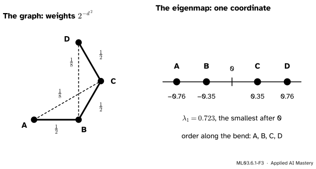
The worked example. Left: the 2-nearest-neighbour graph with weights \({2^{-d^2}}\). Right: the eigenvector of \({\mat{L}\vect{y} = \lambda\mat{D}\vect{y}}\) with the smallest non-zero \(\lambda\) puts the four points on a line in their order round the bend.
Use the symmetry. Swapping \(A \leftrightarrow D\) and \(B \leftrightarrow C\) leaves the graph unchanged, so try \({\vect{y} = (u, v, -v, -u)}\). Write out the rows of \(A\) and \(B\) in \({\mat{L}\vect{y} = \lambda\mat{D}\vect{y}}\), with \({(\mat{L}\vect{y})_i = d_iy_i - \sum_j w_{ij}y_j}\):
\[
\begin{aligned}
\tfrac58 u - \tfrac12 v + \tfrac18 v &= \tfrac58\lambda u, \\
\tfrac98 v - \tfrac12 u + \tfrac12 v + \tfrac18 u &= \tfrac98\lambda v .
\end{aligned}
\]
Times 8, these are \({5u - 3v = 5\lambda u}\) and \({13v - 3u = 9\lambda v}\). The first gives \({v = \tfrac53(1 - \lambda)u}\). Put it into the second and multiply by \({3/u}\):
So \({\lambda = (110 \pm \sqrt{2020})/90}\): 0.723 or 1.722. The other pattern, \({(u, v, v, u)}\), gives \({\lambda = 0}\) (the constant) and \({\lambda = 14/9}\). The smallest non-zero eigenvalue is \({\lambda_1 = 0.723}\), with \({v = \tfrac53 \times 0.277\,u = 0.462\,u}\).
Fix the scale.\({\vect{y}\T\mat{D}\vect{y} = 2(\tfrac58 u^2 + \tfrac98 v^2) = 1}\) gives \({u = 0.760}\) and \({v = 0.351}\). The coordinates are \(0.760\), \(0.351\), \(-0.351\), \(-0.760\) (or all signs flipped; an eigenvector’s sign is arbitrary). The order \(A, B, C, D\) round the bend has become the order along the line.
Code
The worked example first, with scipy.linalg.eigh, which solves \({\mat{L}\vect{y} = \lambda\mat{D}\vect{y}}\) directly when given both matrices.
import numpy as npfrom scipy.linalg import eighdef knn_graph(X, k, sigma):"""Join i and j if either is among the other's k nearest; Gaussian weights on the edges.""" D2 = ((X[:, None, :] - X[None, :, :]) **2).sum(-1) nearest = np.argsort(D2, axis=1)[:, 1:k +1] # column 0 is the point itself A = np.zeros(D2.shape, dtype=bool) A[np.repeat(np.arange(len(X)), k), nearest.ravel()] =True A = A | A.Treturn np.where(A, np.exp(-D2 / (2* sigma **2)), 0.0)def eigenmap(W, q): d = W.sum(axis=1) lam, V = eigh(np.diag(d) - W, np.diag(d), subset_by_index=[0, q])return lam, V[:, 1:] # drop the constant eigenvectorfour = np.array([[0, 0], [1, 0], [1.5, np.sqrt(3) /2], [1, np.sqrt(3)]])W4 = knn_graph(four, 2, 1/ np.sqrt(2* np.log(2)))lam4, y4 = eigenmap(W4, 1)y4 = y4[:, 0] * np.sign(y4[0, 0])print("weights:\n", np.round(W4, 3))print("eigenvalues:", np.round(lam4, 3), " y:", np.round(y4, 3))
Now the swiss roll: 800 points, \(k = 10\), and \(\sigma\) the median distance to the ten nearest neighbours. We check the first coordinate against the hidden position \(t\) with a rank correlation, which is 1 or \(-1\) for a perfect order, and compare with scikit-learn’s SpectralEmbedding, first on our own weights and then with its defaults (no Gaussian: an edge weighs 1 when each point is among the other’s nearest, and ½ when only one is).
from scipy.stats import spearmanrfrom sklearn.datasets import make_swiss_rollfrom sklearn.manifold import SpectralEmbeddingfrom sklearn.neighbors import NearestNeighborsX, t = make_swiss_roll(800, random_state=0)sigma = np.median(NearestNeighbors(n_neighbors=11).fit(X).kneighbors(X)[0][:, 1:])W = knn_graph(X, 10, sigma)lam, Y = eigenmap(W, 2)ours = SpectralEmbedding(2, affinity="precomputed", random_state=0).fit_transform(W)default = SpectralEmbedding(2, n_neighbors=10, random_state=0).fit_transform(X)print("sigma:", round(sigma, 3), " lambda_1:", round(lam[1], 5))print("rank correlation of y_1 with t:", round(abs(spearmanr(Y[:, 0], t)[0]), 4))print("SpectralEmbedding on our weights, |correlation|:", round(abs(np.corrcoef(ours[:, 0], Y[:, 0])[0, 1]), 4))print("SpectralEmbedding defaults, rank correlation with t:", round(abs(spearmanr(default[:, 0], t)[0]), 4))
sigma: 1.89   lambda_1: 0.00076
rank correlation of y_1 with t: 0.9982
SpectralEmbedding on our weights, |correlation|: 1.0
SpectralEmbedding defaults, rank correlation with t: 0.9986
The match with affinity="precomputed" is exact up to sign and scale, because scikit-learn solves the same normalised problem. Spectral clustering on the moons and the circles, where k-means fails (ML03.1.4), scored by the adjusted Rand index against the true groups (1 is perfect, 0 is chance):
from sklearn.cluster import KMeans, SpectralClusteringfrom sklearn.datasets import make_circles, make_moonsfrom sklearn.metrics import adjusted_rand_scoredef spectral_clusters(X, K, k=10): sigma = np.median(NearestNeighbors(n_neighbors=k +1).fit(X).kneighbors(X)[0][:, 1:]) W = knn_graph(X, k, sigma) d = W.sum(axis=1) _, U = eigh(np.eye(len(X)) - W / np.sqrt(np.outer(d, d)), subset_by_index=[0, K -1]) U = U / np.linalg.norm(U, axis=1, keepdims=True) # each row to length 1return KMeans(K, n_init=10, random_state=0).fit_predict(U)scores = {}for name, (Xs, truth) in {"moons": make_moons(200, noise=0.06, random_state=0),"circles": make_circles(200, factor=0.5, noise=0.05, random_state=0)}.items(): km = KMeans(2, n_init=10, random_state=0).fit_predict(Xs) lib = SpectralClustering(2, affinity="nearest_neighbors", n_neighbors=10, random_state=0).fit_predict(Xs) scores[name] = [adjusted_rand_score(truth, lab) for lab in (km, spectral_clusters(Xs, 2), lib)]print(f"{name:8s} k-means {scores[name][0]:.3f} ours {scores[name][1]:.3f} SpectralClustering {scores[name][2]:.3f}")
Last, Isomap from scratch: shortest paths through the graph, then classical MDS.
from scipy.sparse.csgraph import shortest_pathfrom sklearn.manifold import Isomaplengths = np.where(W >0, np.sqrt(((X[:, None] - X[None]) **2).sum(-1)), 0.0)G = shortest_path(lengths, directed=False) # along-the-sheet distancesn =len(X)J = np.eye(n) -1/ nB =-0.5* J @ (G **2) @ J # double centring, as in ML03.5.2ev, vec = eigh(B, subset_by_index=[n -2, n -1])Z = vec[:, ::-1] * np.sqrt(ev[::-1])iso = Isomap(n_neighbors=10, n_components=2).fit_transform(X)print("A to B: straight", round(np.linalg.norm(X[773] - X[674]), 2), " along the graph", round(G[773, 674], 1))print("|correlation| with Isomap:", np.round([abs(np.corrcoef(Z[:, j], iso[:, j])[0, 1]) for j in (0, 1)], 4))print("rank correlation, coordinate 1 with t:", round(abs(spearmanr(Z[:, 0], t)[0]), 4)," coordinate 2 with the height:", round(abs(spearmanr(Z[:, 1], X[:, 1])[0]), 4))
A to B: straight 6.25  along the graph 59.9
|correlation| with Isomap: [1. 1.]
rank correlation, coordinate 1 with t: 0.9999   coordinate 2 with the height: 0.9942
Explore
This module’s interactive, live t-SNE, lives in lesson 3. Its “line” preset is a one-dimensional sheet: watch whether the map keeps its order, the job the eigenmap did here.
Pitfalls
ML03.6.1-F5
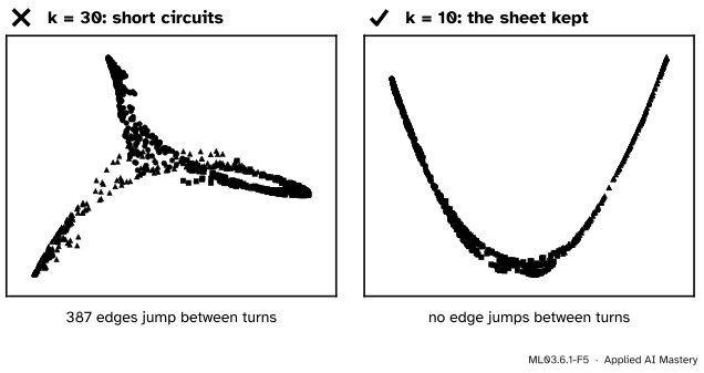
Wrong beside right. With 30 neighbours, 387 edges of the graph jump across the gap to the next turn, and the embedding folds the turns together. With 10, no edge jumps and the order survives.
“More neighbours means a better graph.”
Each extra neighbour is a longer edge, and once edges reach across the gap between two turns they short-circuit the sheet: the graph now says the turns touch. On the swiss roll, SpectralEmbedding with its defaults keeps the order along the sheet at \(k = 10\) (rank correlation 0.999) and loses it at \(k = 30\) (0.10). Too small a \(k\) fails the other way, splitting the graph into pieces: with \(k = 5\) scikit-learn warns that the graph is not connected. Try a few values and check the result, here against \(t\), in practice with the measures of ML03.10.4.
“The second coordinate is the sheet’s other direction.”
On the swiss roll it is not. The sheet is about 89 units long and 21 high, and the smallest eigenvalues belong to slow waves along the long side: the second eigenvector is a wave of double frequency, with an eigenvalue 3.9 times the first, close to the 4 that a long strip predicts. That is why the eigenmap in the opening figure is a U, not a rectangle. Isomap, which keeps distances rather than only neighbourhoods, does return the rectangle.
“Spectral clustering finds the right number of clusters.”
It needs \(K\), like k-means. The gap after the \(K\)-th smallest eigenvalue is a useful hint (a graph in \(K\) separate pieces has exactly \(K\) zero eigenvalues, M03.9.3), but on real data the gap is often unclear, and the choice is judged as in ML03.10.
Check yourself
Recall
1. Which pairs of points does a k-nearest-neighbour graph join?
Show answer
Points \(i\) and \(j\) are joined when either is among the other’s \(k\) nearest neighbours, so the graph is symmetric.
2. Write the spring energy of an embedding \(\vect{y}\) as a quadratic form.
3. What eigenproblem gives the Laplacian eigenmap, and which eigenvector is dropped?
Show answer
\({\mat{L}\vect{y} = \lambda\mat{D}\vect{y}}\). The constant vector, with \(\lambda = 0\), is dropped; the next \(q\) eigenvectors are the coordinates.
4. What are the steps of spectral clustering after the graph is built?
Show answer
Take the \(K\) smallest eigenvectors of the normalised Laplacian, rescale each row to length 1, and run k-means on the rows.
5. What goes wrong when \(k\) is too large on the swiss roll?
Show answer
Edges reach across the gap between turns and short-circuit the sheet, so the embedding folds the turns together: 387 such edges at \(k = 30\).
Exercises
1.★ Three points sit on a line at 0, 1 and 3, and the graph joins 0–1 with weight \({w = 0.6}\) and 1–3 with weight \({w = 0.1}\). Write \(\mat{W}\), \(\mat{D}\) and \(\mat{L}\), and evaluate the spring energy of \({\vect{y} = (-1, 0, 1)}\).
Show solution
\(\mat{W}\) has 0.6 in positions (1, 2) and (2, 1), and 0.1 in positions (2, 3) and (3, 2). The degrees are 0.6, 0.7 and 0.1, so \({\mat{D} = \operatorname{diag}(0.6, 0.7, 0.1)}\), and \(\mat{L}\) has rows \({(0.6, -0.6, 0)}\), \({(-0.6, 0.7, -0.1)}\) and \({(0, -0.1, 0.1)}\). The energy sums over ordered pairs, so each edge counts twice: \({2\,(0.6 \times 1^2 + 0.1 \times 1^2) = 1.4}\). As a check, \({2\,\vect{y}\T\mat{L}\vect{y} = 2\,(0.6 + 0.1) = 1.4}\).
2.★★ Four points form a path, \(A\)–\(B\)–\(C\)–\(D\), every edge with weight 1. Show that \({\vect{y} = (1, \tfrac12, -\tfrac12, -1)}\) solves \({\mat{L}\vect{y} = \lambda\mat{D}\vect{y}}\) and find \(\lambda\). Compare with the worked example.
Show solution
The degrees are 1, 2, 2, 1. Row \(A\): \({y_A - y_B = \tfrac12}\), and \({\lambda d_A y_A = \lambda}\), so \({\lambda = \tfrac12}\). Row \(B\): \({2y_B - y_A - y_C = 1 - 1 + \tfrac12 = \tfrac12}\), and \({\lambda d_B y_B = \tfrac12 \times 2 \times \tfrac12 = \tfrac12}\). Rows \(C\) and \(D\) follow by symmetry. So \({\lambda = \tfrac12}\). In the worked example the two skip edges \(AC\) and \(BD\) tie the ends to the middle, which raises \(\lambda_1\) to 0.723 and draws \(B\) and \(C\) in to \({\pm 0.462}\) times the ends’ value instead of \({\pm 0.5}\).
3.★★★ Prove that if the graph falls into two pieces with no edge between them, the eigenproblem has a second eigenvector with \({\lambda = 0}\), and describe it. What does that say about the eigenmap of a disconnected graph?
Show solution
Let \(S\) be one piece, and let \(\vect{y}\) be \({a}\) on \(S\) and \({b}\) elsewhere, with \({a \ne b}\). Every edge joins two points of the same piece, so every term \({w_{ij}(y_i - y_j)^2}\) is zero and \({\vect{y}\T\mat{L}\vect{y} = 0}\). As \(\mat{L}\) is positive semidefinite, a vector with \({\vect{y}\T\mat{L}\vect{y} = 0}\) satisfies \({\mat{L}\vect{y} = \vect{0} = 0 \cdot \mat{D}\vect{y}}\). Choosing \(a\) and \(b\) so that \({\vect{y}\T\mat{D}\vect{1} = 0}\) meets the second guard, so this step vector is an eigenvector with \({\lambda = 0}\) besides the constant. The eigenmap then just reports which piece each point is in, two values and no shape, which is why Belkin and Niyogi embed each connected piece separately.
Summary card
Trust only short distances, and let eigenvectors lay the graph out.
Eigenmap.\({\mat{L}\vect{y} = \lambda\mat{D}\vect{y}}\); skip \({\lambda_0 = 0}\), keep the next \(q\).
Spectral clustering. Rows of the bottom \(K\) eigenvectors, normalised, then k-means.
Choose k with care. Too large short-circuits; too small disconnects.
Sources and next steps
Sources. Each was opened and checked against this lesson on 15 November 2026.
Mikhail Belkin and Partha Niyogi, Laplacian Eigenmaps for Dimensionality Reduction and Data Representation, Neural Computation 15 (2003). Section 2 gives the algorithm: an edge if either point is among the other’s \(n\) nearest neighbours, heat-kernel weights \({e^{-\norm{x_i - x_j}^2/t}}\) (our \({t = 2\sigma^2}\)), and the generalised eigenproblem \({Lf = \lambda Df}\) (2.1) with the eigenvector of eigenvalue 0 left out. Section 3.1 derives \({\tfrac12\sum_{i,j}(y_i - y_j)^2W_{ij} = y\T Ly}\) (3.1) and the constraints \({y\T Dy = 1}\) and \({y\T D\vect{1} = 0}\).
Andrew Ng, Michael Jordan and Yair Weiss, On Spectral Clustering: Analysis and an algorithm, NeurIPS 14 (2001), Section 2. The algorithm: Gaussian affinities, the matrix \({D^{-1/2}AD^{-1/2}}\) and its \(k\) largest eigenvectors (the smallest of the normalised Laplacian), rows renormalised to unit length, then k-means on the rows.
scikit-learn 1.9 User Guide, Section 2.2, Manifold learning. Section 2.2.6 describes SpectralEmbedding as Laplacian eigenmaps (affinity graph, Laplacian \({L = D - A}\) or its normalised form, partial eigendecomposition); Section 2.2.2 describes Isomap as a neighbour search, a shortest-path search and an eigendecomposition.
Next.ML03.6.2 From SNE to t-SNE keeps the idea of trusting neighbours but turns distances into probabilities, which makes clusters stand out far more clearly.