Judge each point against its own neighbourhood: the local outlier factor compares a point’s density with its neighbours’ densities. Build it from k-distance, reachability distance and local reachability density, compute it by hand on the twelve points, and use it in scikit-learn.
ML03.9.2L2 Intermediate30 minIn review (what this means)
The maths and code on this page are checked by automated tests on every change, but an independent reader has not signed it off yet. Spot a mistake or a confusing step? Tell us.
Use the distance to the k-th neighbour as an anomaly score, and explain why it fails when clusters have different densities.
Define the k-distance, the reachability distance, the local reachability density and the local outlier factor.
Compute the local outlier factor by hand on the twelve points with k = 3, getting 1.597 for the bridge and 3.514 for (9, 1).
Match a from-scratch LOF with sklearn.neighbors.LocalOutlierFactor, and score new points with novelty=True.
The question
A payment of 300 is routine for a customer who spends thousands a month and alarming for one who never spends more than 20. One global yardstick cannot serve both. The Mahalanobis distance of the last lesson fits one cloud to everybody. Can a score judge each point against its own neighbourhood instead?
From the last lesson
1. What two steps does every anomaly detector take?
Show answer
It scores every point by how strange it is, then flags the points whose score reaches a threshold \(c\), often chosen so that a share equal to the expected contamination is flagged.
2. Why did the single Gaussian call the bridge point \((4.5, 3.5)\) the most typical of the twelve points?
Show answer
One Gaussian fitted to two groups puts its mean, and its peak density, between them, which is exactly where the bridge sits: its \({D^2}\) is only 0.025.
Intuition
Look at how crowded each point’s neighbourhood is, and compare it with how crowded its neighbours’ neighbourhoods are. A point in a sparse cloud is fine if its neighbours live just as sparsely. A point is strange when it is much lonelier than the points around it.
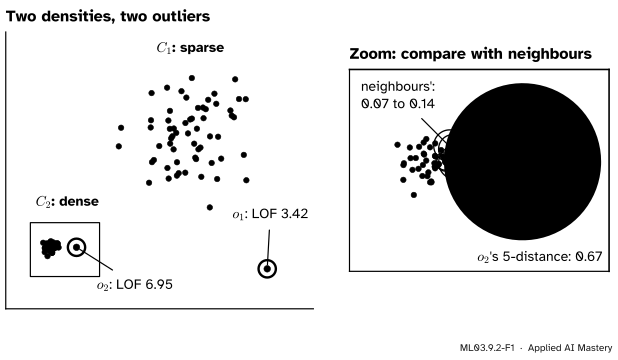
ML03.9.2-F1
The outlier \(o_2\) is closer to its neighbours than many normal points of the sparse cloud \(C_1\) are to theirs. What gives it away is the comparison: its neighbourhood is about six times wider than the neighbourhoods of the points it is near.
This is the local outlier factor (LOF) of Breunig, Kriegel, Ng and Sander (2000). The data set in the picture follows the example of their section 3 on a smaller scale: a sparse cluster \(C_1\), a dense cluster \(C_2\), and two outliers. Any score that measures distance on one global scale must either call \(o_2\) normal or call many points of \(C_1\) strange. A ratio of local densities does neither.
Build it up
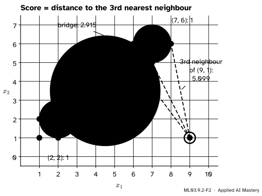
Step 1. Distance to the k-th neighbour. The simplest local score is how far a point must reach to find \(k\) other points. On the twelve points with \(k = 3\) the groups need 1 to 2, the bridge 2.915 and the far point 5.099.
ML03.9.2-F2
The distance to the third nearest neighbour. Inside the groups it is 1 to 2; the bridge must reach 2.915 and the far point 5.099.
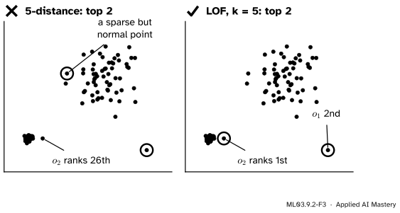
Step 2. Where it fails. In the two-density data of the anchor figure, take \(k = 5\). The outlier \(o_2\) has its fifth neighbour 0.67 away. Twenty-five points of the sparse cloud reach further, so \(o_2\) ranks 26th.
ML03.9.2-F3
One yardstick for all fails: the 5-distance flags a normal point of the sparse cloud and ranks \(o_2\) only 26th. LOF puts \(o_2\) first and \(o_1\) second.
Step 3. Turn distance into density and compare. Reaching far to find \(k\) neighbours means low density. Invert an average reach to get a density, then divide the neighbours’ densities by the point’s own. A ratio near 1 says “as crowded as my neighbours”; a large ratio says “much sparser”.
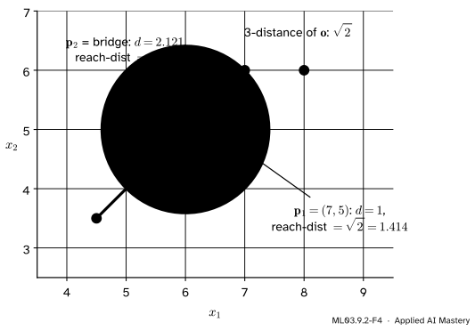
Step 4. Smooth the distances. Inside a tight group, distances between near neighbours jump about by chance, and so would their inverses. Breunig and colleagues replace a short distance by a floor: the neighbour’s own \(k\)-distance.
ML03.9.2-F4
The reachability distance. A point inside \(\vect{o}\)’s circle is given the circle’s radius; a point outside keeps its true distance.
The formal statement
Fix a whole number \(k\) (“MinPts” in the paper, n_neighbors in scikit-learn) and a distance \(d\). The definitions follow Breunig et al. (2000, section 4, Definitions 3 to 7). Throughout, \(N_k(\vect{p})\) is the set of the \(k\) nearest neighbours of \(\vect{p}\), not counting \(\vect{p}\).
NoteDefinitions: the local outlier factor
The \(k\)-distance of \(\vect{o}\) is the distance from \(\vect{o}\) to its \(k\)-th nearest neighbour.
The reachability distance of \(\vect{p}\) from \(\vect{o}\) is the true distance, but never less than \(\vect{o}\)’s own \(k\)-distance.
The local reachability density of \(\vect{p}\) is one over its mean reachability distance.
The local outlier factor of \(\vect{p}\) is the mean ratio of its neighbours’ densities to its own.
In symbols, with \({N = N_k(\vect{p})}\) and \({\abs{N} = k}\):
Since \(\operatorname{lrd}_k(\vect{p})\) is the same in every term, the second formula is simply the neighbours’ mean density divided by the point’s own.
Deep inside a cluster, LOF is close to 1. Lemma 1 of the paper makes this precise. Let the reachability distances within a cluster lie between a smallest value \(r_{\min}\) and a largest \(r_{\max}\), and let \(\vect{p}\) be deep inside it (its neighbours, and theirs, all in the cluster). Then every average of reachability distances also lies between \(r_{\min}\) and \(r_{\max}\), so every lrd involved lies between \(1/r_{\max}\) and \(1/r_{\min}\). A ratio of two such numbers lies between \(r_{\min}/r_{\max}\) and \(r_{\max}/r_{\min}\). In a tight cluster those two are close, so LOF is close to 1. That is why there is no need to know the cluster’s density: LOF measures it in its own units.
The scale cancels. Multiply every distance by a factor \(a > 0\). Every \(k\)-distance and every reachability distance is multiplied by \(a\), so every lrd is divided by \(a\), and in the ratio the \(a\) cancels. LOF does not change. A raw \(k\)-distance would change by the factor \(a\).
Go deeper: ties, and why some libraries give other numbers
The paper’s \(k\)-distance neighbourhood holds every point within the \(k\)-distance, so with ties it can hold more than \(k\) points (Definition 4). scikit-learn takes exactly \(k\) neighbours, and on a tie it keeps the points that come first in the data. The twelve points sit on a grid, so ties are common: the bridge has three points at distance 2.915. With the paper’s definition the bridge scores 1.807 and \((9, 1)\) scores 3.356 instead of 1.597 and 3.514. The ranking is the same. Both conventions are honest; say which one you use.
Worked example
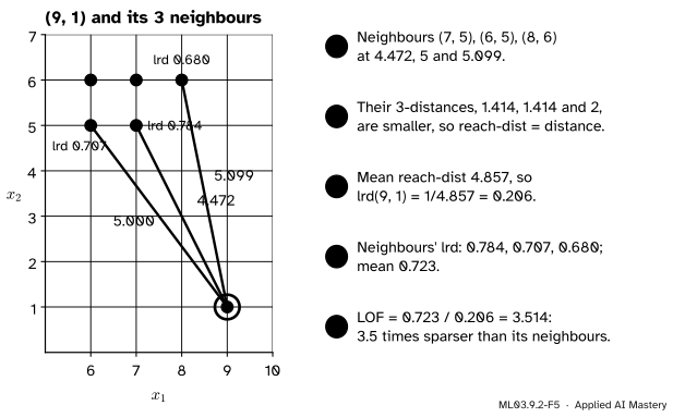
The twelve points with \(k = 3\). First the 3-distances, read from the sorted distances of each point: 1.414 for \((1, 1)\), \((2, 1)\), \((1, 2)\), \((6, 5)\), \((7, 5)\) and \((6, 6)\); 1 for \((2, 2)\) and \((7, 6)\); 2 for \((3, 2)\) and \((8, 6)\); 2.915 for the bridge; 5.099 for \((9, 1)\).
ML03.9.2-F5
The local outlier factor of \((9, 1)\) with \(k = 3\), step by step.
The far point \((9, 1)\). Its three nearest neighbours are \((7, 5)\), \((6, 5)\) and \((8, 6)\), at \({\sqrt{20} = 4.472}\), \({\sqrt{25} = 5}\) and \({\sqrt{26} = 5.099}\). Their 3-distances are all smaller, so each reachability distance is the true distance. The mean is \({(4.472 + 5 + 5.099)/3 = 4.857}\), so \({\operatorname{lrd}(9, 1) = 1/4.857 = 0.206}\).
Its neighbours’ densities. For \((6, 5)\), the neighbours \((7, 5)\), \((6, 6)\) and \((7, 6)\) are at 1, 1 and 1.414, with 3-distances 1.414, 1.414 and 1, so each reachability distance is 1.414 and \({\operatorname{lrd} = 1/1.414 = 0.707}\). In the same way \((7, 5)\) has reachability distances 1.414, 1 and 1.414, giving \({\operatorname{lrd} = 1/1.276 = 0.784}\), and \((8, 6)\) has 1, 1.414 and 2, giving \({\operatorname{lrd} = 1/1.471 = 0.680}\).
The factor. The neighbours’ mean density is \({(0.784 + 0.707 + 0.680)/3 = 0.723}\), and
The bridge \((4.5, 3.5)\). Its neighbours are \((3, 2)\) and \((6, 5)\) at 2.121, and \((2, 2)\) at 2.915 (tied with two others, taken in list order). The reachability distances are \({\max(2, 2.121) = 2.121}\), \({\max(1.414, 2.121) = 2.121}\) and \({\max(1, 2.915) = 2.915}\), with mean 2.386, so \({\operatorname{lrd} = 0.419}\). The neighbours’ densities are 0.680, 0.707 and 0.621, with mean 0.669, so \({\operatorname{LOF} = 0.669/0.419 = 1.597}\).
Result:\((9, 1)\) scores 3.514 and the bridge 1.597. The ten group points score between 0.898 and 1.205, close to 1, as Lemma 1 predicts.
Code
From scratch, with exactly \(k\) neighbours and ties broken by order, as scikit-learn does.
import numpy as npX = np.array([(1, 1), (2, 1), (1, 2), (2, 2), (3, 2), (6, 5), (7, 5), (6, 6), (7, 6), (8, 6), (4.5, 3.5), (9, 1)], dtype=float)def lof(X, k): D = np.sqrt(((X[:, None, :] - X[None, :, :]) **2).sum(axis=-1)) nb = np.argsort(D, axis=1, kind="stable")[:, 1:k +1] # k nearest, without the point kdist = D[np.arange(len(X)), nb[:, -1]] # distance to the k-th reach = np.maximum(kdist[nb], D[np.arange(len(X))[:, None], nb]) lrd =1/ reach.mean(axis=1)return kdist, lrd, lrd[nb].mean(axis=1) / lrdkdist, lrd, factor = lof(X, k=3)print("3-distances:", kdist.round(3))print("lrd:", lrd.round(3))print("LOF:", factor.round(3))
scikit-learn stores minus the factor in negative_outlier_factor_. With the default contamination="auto", a point is flagged when its LOF exceeds 1.5.
from sklearn.neighbors import LocalOutlierFactormodel = LocalOutlierFactor(n_neighbors=3)labels = model.fit_predict(X)print("matches from scratch:", np.allclose(-model.negative_outlier_factor_, factor))print("flagged (-1):", X[labels ==-1].tolist())
matches from scratch: True
flagged (-1): [[4.5, 3.5], [9.0, 1.0]]
For novelty detection, fit on clean data with novelty=True and score only new points.
clean = LocalOutlierFactor(n_neighbors=3, novelty=True).fit(X[:10])new = np.array([(4.5, 3.5), (9, 1), (4, 3), (2.5, 1.5)])print("LOF of new points:", (-clean.score_samples(new)).round(3))
LOF of new points: [1.597 3.514 1.636 1.022]
The bridge and \((9, 1)\) keep their scores: neither was among anybody’s three nearest neighbours, so removing them changes no other density. The point \((2.5, 1.5)\), inside the lower group, scores 1.022.
Explore
This module’s interactive lives in ML03.9.3. It scores points by isolation instead of density; drag its chosen point between the two blobs and compare how the two ideas treat a point that sits in a gap.
Pitfalls
ML03.9.2-F6
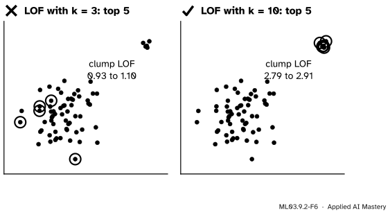
Wrong beside right. With \(k = 3\), each point of a clump of five finds its neighbours inside the clump and looks normal. With \(k = 10\) the neighbourhoods reach the main cloud, and the clump stands out.
“A small k keeps LOF local, so smaller is better.”
If \(k\) is smaller than a group of anomalies, they are each other’s neighbours and vouch for one another. Pick \(k\) larger than the largest clump of anomalies you need to catch. scikit-learn’s guide finds 20 works well in general and suggests more when over a tenth of the data may be anomalous.
“LOF above 1 means anomaly.”
LOF is a ratio, not a probability. Normal points scatter around 1 (here 0.898 to 1.205), and how far above 1 counts as strange depends on the data. scikit-learn’s default cut of 1.5 is a convention; ranking, or a contamination you can defend, is safer.
“With novelty=True, score the training data too.”
A training point is its own nearest neighbour at distance 0, so its novelty score is biased. scikit-learn’s guide says to use predict, decision_function and score_samples only on new data, and turns fit_predict off in this mode.
Check yourself
Recall
1. Why does the distance to the \(k\)-th neighbour fail as a score when clusters have different densities?
Show answer
It measures every point on one global scale. A point just outside a dense cluster can be closer to its neighbours than ordinary points of a sparse cluster are to theirs, so it ranks below them.
2. Define the reachability distance of \(\vect{p}\) from \(\vect{o}\).
Show answer
The larger of \(\vect{o}\)’s \(k\)-distance and the true distance \({d(\vect{p}, \vect{o})}\): the true distance, but never less than \(\vect{o}\)’s own \(k\)-distance.
3. What value does LOF take for a point deep inside a cluster, and why?
Show answer
Close to 1. Its density and its neighbours’ densities are built from reachability distances of the same cluster, so their ratio lies between \(r_{\min}/r_{\max}\) and \(r_{\max}/r_{\min}\) (Lemma 1).
4. What are the LOF scores of the bridge and of \((9, 1)\) with \(k = 3\)?
Show answer
1.597 for the bridge \((4.5, 3.5)\) and 3.514 for \((9, 1)\).
5. What does negative_outlier_factor_ hold, and what changes with novelty=True?
Show answer
Minus the LOF of each training point. With novelty=True, score_samples and predict become available for new points, and fit_predict does not.
Exercises
1.★ Compute the local reachability density of \((2, 2)\) with \(k = 3\). Its neighbours are \((3, 2)\), \((2, 1)\) and \((1, 2)\), each at distance 1.
Show solution
The 3-distances of the neighbours are 2 for \((3, 2)\) and 1.414 for \((2, 1)\) and \((1, 2)\). The reachability distances are \({\max(2, 1) = 2}\), \({\max(1.414, 1) = 1.414}\) and \({\max(1.414, 1) = 1.414}\). Their mean is \({4.828/3 = 1.609}\), so \({\operatorname{lrd}(2, 2) = 1/1.609 = 0.621}\). Note that every true distance is 1, yet the floor raises the average: the smoothing at work.
2.★★ Every coordinate of the twelve points is multiplied by 10. What happens to the 3-distance of \((9, 1)\), to its lrd and to its LOF?
Show solution
All distances are multiplied by 10, so the 3-distance becomes 50.99. Every reachability distance is multiplied by 10 too, so every lrd is divided by 10: \({\operatorname{lrd}(90, 10) = 0.0206}\). The LOF is a ratio of two lrds, so the factor 10 cancels: it stays 3.514.
3.★★★ Show that \({\operatorname{LOF}_k(\vect{p}) \ge r_{\min}/r_{\max}}\), where \(r_{\min}\) is the smallest reachability distance from \(\vect{p}\) to its neighbours and \(r_{\max}\) the largest reachability distance from any neighbour \(\vect{o}\) of \(\vect{p}\) to a neighbour of \(\vect{o}\). (This is half of Theorem 1 of Breunig et al.)
Show solution
Every reachability distance from \(\vect{p}\) is at least \(r_{\min}\), so their mean is at least \(r_{\min}\), and \({\operatorname{lrd}(\vect{p}) \le 1/r_{\min}}\).
For each neighbour \(\vect{o}\), every reachability distance from \(\vect{o}\) to its own neighbours is at most \(r_{\max}\), so their mean is at most \(r_{\max}\), and \({\operatorname{lrd}(\vect{o}) \ge 1/r_{\max}}\).
and a mean of numbers that are all at least \(r_{\min}/r_{\max}\) is at least \(r_{\min}/r_{\max}\). For \((9, 1)\), \({r_{\min} = 4.472}\) and \({r_{\max} = 2}\) (the largest reachability distance among its neighbours’ neighbourhoods), so LOF is at least 2.236; it is 3.514.
Summary card
A point is anomalous when it is much sparser than its own neighbours.
ML03.9.2-F1
Compare with the neighbours.
Reach. The distance from \(\vect{p}\) to \(\vect{o}\), floored at \(\vect{o}\)’s \(k\)-distance.
Density.\(\operatorname{lrd}_k(\vect{p})\): one over the mean reachability distance to the \(k\) neighbours.
Factor.\(\operatorname{LOF}_k(\vect{p})\): neighbours’ mean lrd over the point’s own; about 1 inside a cluster.
Twelve points, \(k = 3\). Bridge 1.597, \((9, 1)\) 3.514, groups 0.898 to 1.205.
In code.LocalOutlierFactor(n_neighbors=k): negative_outlier_factor_; novelty=True for new points.
Sources and next steps
Sources. Each was opened and checked against this lesson on 15 November 2026.
Markus M. Breunig, Hans-Peter Kriegel, Raymond T. Ng and Jörg Sander, LOF: identifying density-based local outliers, Proceedings of ACM SIGMOD 2000, pages 93 to 104 (a copy kept by Florida Institute of Technology). Section 3 and Figure 1 give the example of a sparse cluster, a dense cluster and the outliers \(o_1\) and \(o_2\); section 4 gives Definitions 3 to 7 (\(k\)-distance, the \(k\)-distance neighbourhood that may hold more than \(k\) points, reachability distance, lrd and LOF); section 5.1 gives Lemma 1 and section 5.2 Theorem 1, whose lower bound is exercise 3.
scikit-learn developers, User Guide, sections 2.7.3.3 and 2.7.4, version 1.9: n_neighbors=20 works well in general, more when the share of outliers is high; in novelty mode use predict, decision_function and score_samples only on new data.
scikit-learn developers, sklearn.neighbors.LocalOutlierFactor: negative_outlier_factor_ is the opposite of LOF, inliers score near \(-1\), and offset_ is \(-1.5\) when contamination="auto".
Next.ML03.9.3 Isolation forests measures no distances at all: it asks how many random cuts it takes to fence a point off on its own.