Instead of one eps, OPTICS orders the points so that each comes after its densest neighbour and records a reachability distance. Read clusters at every density as valleys of the reachability plot, recover DBSCAN for any eps with one horizontal line, and build it with a priority queue.
ML03.3.3L2 Intermediate30 minIn review (what this means)
The maths and code on this page are checked by automated tests on every change, but an independent reader has not signed it off yet. Spot a mistake or a confusing step? Tell us.
Define the core distance and the reachability distance, and compute them on the twelve points.
Run the OPTICS ordering by hand on the twelve points, choosing next the unprocessed point of smallest reachability.
Read a reachability plot: valleys are clusters, and a horizontal line at eps recovers the DBSCAN clustering for that eps.
Build OPTICS from scratch with a priority queue (heapq) and match sklearn.cluster.OPTICS and cluster_optics_dbscan.
The question
In the last lesson no single eps could serve two tight blobs and one sparse one: small values dissolved the sparse blob, large values merged the tight ones. Each eps is one horizontal slice through the data’s density. Could one pass over the data record every slice at once, so that you can look at all densities together and decide afterwards?
From the last lesson
1. With min_samples = m, when exactly is a point core?
Show answer
When its distance to its \((m - 1)\)-th nearest other point is at most \(\varepsilon\).
2. As eps grows with min_samples fixed, what can happen to two clusters of core points?
Show answer
They can merge, but they never split: core points stay core and their edges stay edges.
Intuition
Walk through the data, always stepping next to the unvisited point that is easiest to reach from where you have been. Inside a crowd every step is short. When the crowd is used up, the next step must cross open ground, and it is long. Write down the length of each step as you go, and the crowds appear as runs of short steps between long ones.
ML03.3.3-F1
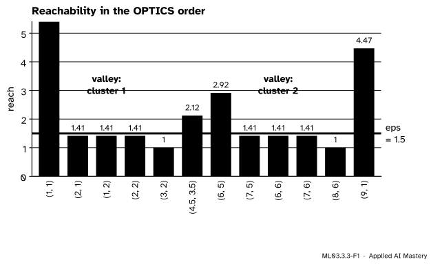
The reachability plot of the twelve points with min_samples = 4. Each bar is how hard it was to reach that point. The valleys are the two clusters; a line at \(\varepsilon = 1.5\) leaves the bridge and \((9, 1)\) above it as noise, exactly as DBSCAN did.
This is OPTICS (ordering points to identify the clustering structure) of Ankerst, Breunig, Kriegel and Sander (1999). It does not return clusters. It returns an ordering of the points and a reachability distance for each, and from those two you can read the clusters for any \(\varepsilon\) you like: a valley that stays below a line is a cluster at that density.
Build it up
Keep min_samples\(= m = 4\) throughout.
Step 1. The core distance. The core distance of a point \(\vect{p}\) is the smallest radius at which it would be a core point: its distance to its \((m - 1)\)-th nearest other point, the k-distance of the last lesson. For the bridge \((4.5, 3.5)\) it is \(\sqrt{8.5} \approx 2.915\).
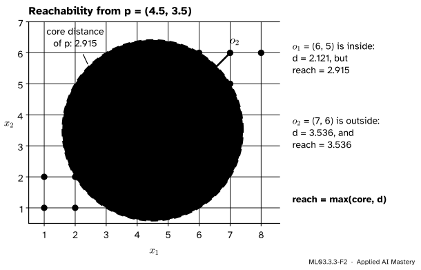
Step 2. The reachability distance. How far is \(\vect{o}\) from a core point \(\vect{p}\), as far as density goes? If \(\vect{o}\) lies inside the core circle of \(\vect{p}\), it is reachable as soon as \(\vect{p}\) is core, so its distance counts as the core distance. If it lies outside, it counts as the plain distance. Together: the reachability distance of \(\vect{o}\) from \(\vect{p}\) is the larger of the core distance of \(\vect{p}\) and the distance from \(\vect{p}\) to \(\vect{o}\).
ML03.3.3-F2
Reachability from the bridge \(\vect{p}\). Its core distance is 2.915. A point inside the core circle, such as \(o_1 = (6, 5)\) at distance 2.121, gets reachability 2.915; a point outside, such as \(o_2 = (7, 6)\) at distance 3.536, keeps its distance.
Taking the larger of the two smooths away the fine detail inside a dense region: every point within the core circle of \(\vect{p}\) is equally easy to reach from it.
Step 3. The ordering. Start at the first point. Repeat: for every point not yet visited, lower its reachability to the reachability from the point just visited, if that is smaller; then visit next the unvisited point with the smallest reachability. Keep the unvisited points in a priority queue keyed by reachability, so that the next one is always at the front.
Step 4. The plot. Draw one bar per point, in visiting order, as tall as its reachability when it was visited. A dense cluster is a run of low bars, a valley; the first point of each new region, reached only across a gap, is a high bar.
The formal statement
Let \(\vect{p}\) have \(m - 1\) nearest other points with the largest of their distances \(d_{m-1}(\vect{p})\). With no upper limit on \(\varepsilon\) (scikit-learn’s default max_eps=inf), the two quantities of Ankerst et al. (section 3.2.1, Definitions 5 and 6) are
By the proposition of the last lesson, \(\vect{p}\) is core for \(\varepsilon\) exactly when \(\operatorname{core}(\vect{p}) \le \varepsilon\). So \(\operatorname{reach}_{\vect{p}}(\vect{o}) \le \varepsilon\) says two things at once: \(\vect{p}\) is core at \(\varepsilon\), and \(\vect{o}\) lies within \(\varepsilon\) of it. In other words, the reachability distance is the smallest \(\varepsilon\) at which \(\vect{o}\) is directly density-reachable from \(\vect{p}\).
NoteThe OPTICS ordering
Set every reachability to \(\infty\). While points remain unvisited: visit the unvisited point \(\vect{p}\) with the smallest reachability (the first in the data if all are \(\infty\)), and for every unvisited \(\vect{o}\) set
The output is the visiting order and, for each point, \(r\) at the moment it was visited. The point that last lowered \(r(\vect{o})\) is its predecessor.
So the recorded reachability of a point is the smallest \(\varepsilon\) at which it is directly reachable from some point visited before it.
NoteReading off DBSCAN (ExtractDBSCAN-Clustering, Ankerst et al., Figure 8)
For any \(\varepsilon'\), scan the points in order. If \(r(\vect{p}) > \varepsilon'\): start a new cluster at \(\vect{p}\) when \(\operatorname{core}(\vect{p}) \le \varepsilon'\), otherwise mark it noise. If \(r(\vect{p}) \le \varepsilon'\): put it in the current cluster. The result is the DBSCAN clustering for \(\varepsilon'\), except perhaps for a few border points.
Why it works: a bar at or below \(\varepsilon'\) means the point is directly reachable at \(\varepsilon'\) from an earlier point (exercise 3), so it belongs with what came before. A bar above \(\varepsilon'\) means no earlier point reaches it, so it starts something new: a cluster if it is core, noise if not. And the walk finishes each cluster before it leaves it (see the collapsed proof below).
ML03.3.3-F4
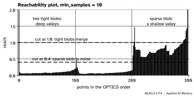
The blobs of two densities, with min_samples = 10. The tight blobs are deep valleys and the sparse blob a shallow one. A line at 0.4 cuts the sparse valley away as noise; a line at 1.0 is above the small bar between the tight blobs, so it merges them.
Nested structure shows too: the two tight valleys sit inside a larger region whose bars are all below 1.0. Lowering \(\varepsilon\) splits a cluster into the denser clusters inside it.
Go deeper: why the walk finishes one cluster before it starts the next
Fix \(\varepsilon'\) and let \(C\) be the set of core points (at \(\varepsilon'\)) of one DBSCAN cluster. Suppose the walk has visited some point of \(C\) but not all of them. Because \(C\) is connected in the core graph, some visited \(\vect{a} \in C\) is within \(\varepsilon'\) of some unvisited \(\vect{b} \in C\). Both are core, so \(\operatorname{reach}_{\vect{a}}(\vect{b}) \le \varepsilon'\), and therefore \(r(\vect{b}) \le \varepsilon'\) from the moment \(\vect{a}\) was visited.
The walk always takes the smallest \(r\). So before it takes any point with \(r > \varepsilon'\), it takes points with \(r \le \varepsilon'\), each of which is directly reachable at \(\varepsilon'\) from a visited point. If that visited point lies in \(C\)’s cluster, so does the new point (it is either in \(C\) or one of its border points). The walk can only reach outside the cluster through a point with \(r \le \varepsilon'\) that is directly reachable from a core point of \(C\), and such a point is a border point of \(C\)’s cluster. So all of \(C\) is visited, with bars at most \(\varepsilon'\), before any bar above \(\varepsilon'\) appears. The only slack is a border point shared with another cluster: it may be visited with the wrong cluster, which is the “few border points” of the statement.
Worked example
OPTICS on the twelve points with min_samples = 4. The core distances are the 3-distances of the last lesson: 1.414 for six corners, 1 for \((2, 2)\) and \((7, 6)\), 2 for \((3, 2)\) and \((8, 6)\), 2.915 for the bridge and 5.099 for \((9, 1)\).
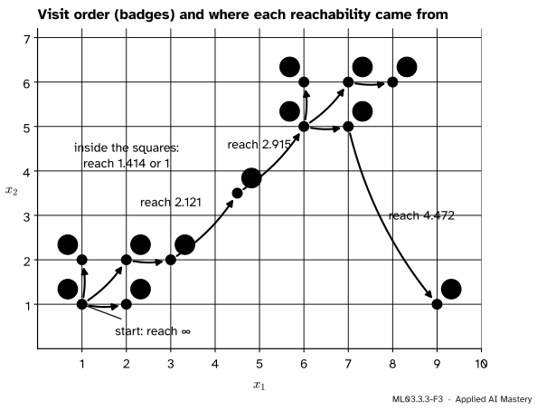
Steps 1 to 5. Start at \((1, 1)\), with \(r = \infty\). Its core distance is 1.414, so it gives \(r = \max(1.414, 1) = 1.414\) to \((2, 1)\) and \((1, 2)\), \(\max(1.414, 1.414) = 1.414\) to \((2, 2)\), and \(\max(1.414, 2.236) = 2.236\) to \((3, 2)\). Three points tie at 1.414; take them in data order: \((2, 1)\), which lowers \((3, 2)\) to \(\max(1.414, 1.414) = 1.414\), then \((1, 2)\), then \((2, 2)\). The corner \((2, 2)\) has core distance 1, so it lowers \((3, 2)\) to \(\max(1, 1) = 1\). Visit \((3, 2)\).
Steps 6 and 7. The cheapest unvisited point is now the bridge, reached from \((3, 2)\) with \(\max(2, 2.121) = 2.121\). Its core distance is 2.915, so from it \((6, 5)\) costs \(\max(2.915, 2.121) = 2.915\), cheaper than the 4.243 offered from \((3, 2)\). Visit \((6, 5)\) at 2.915.
Steps 8 to 12. The upper square repeats the lower one: three points at 1.414, then \((8, 6)\) at 1, reached from \((7, 6)\). Last comes \((9, 1)\), cheapest from \((7, 5)\) at \(\max(1.414, 4.472) = 4.472\).
ML03.3.3-F3
The walk. Badges give the visit order; each arrow comes from the point that set the reachability. Only three steps cross open ground: to the bridge, to the upper square and to \((9, 1)\).
step
point
reach
set by
1
\((1, 1)\)
\(\infty\)
2 to 4
three corners
1.414
\((1, 1)\)
5
\((3, 2)\)
1
\((2, 2)\)
6
\((4.5, 3.5)\)
2.121
\((3, 2)\)
7
\((6, 5)\)
2.915
bridge
8 to 10
three corners
1.414
\((6, 5)\)
11
\((8, 6)\)
1
\((7, 6)\)
12
\((9, 1)\)
4.472
\((7, 5)\)
Reading it. With the line at \(\varepsilon' = 1.5\): \((1, 1)\) is above but core (1.414), so it starts cluster 1; the next four are below and join it. The bridge is above and not core (2.915): noise. \((6, 5)\) is above but core: it starts cluster 2, and four more join. \((9, 1)\) is above and not core: noise. That is DBSCAN’s answer. At \(\varepsilon' = 2.5\) the bridge’s bar (2.121) is below the line, so it joins cluster 1, as DBSCAN gave it in the last lesson. At \(\varepsilon' = 3\) the bar of \((6, 5)\) (2.915) is below too, and everything but \((9, 1)\) is one cluster.
Code
From scratch, with Python’s heapq as the priority queue. An entry whose reachability has since been lowered stays in the heap; it is skipped when it comes out after the point is already visited.
import heapqimport numpy as npfrom sklearn.cluster import OPTICS, DBSCAN, cluster_optics_dbscanX = np.array([(1, 1), (2, 1), (1, 2), (2, 2), (3, 2), (6, 5), (7, 5), (6, 6), (7, 6), (8, 6), (4.5, 3.5), (9, 1)], dtype=float)def optics(X, min_samples): D = np.sqrt(((X[:, None, :] - X[None, :, :]) **2).sum(axis=-1)) core = np.sort(D, axis=1)[:, min_samples -1] # column 0 is the point itself n =len(X) reach, pred = np.full(n, np.inf), np.full(n, -1) done, order = np.zeros(n, dtype=bool), []for start inrange(n):if done[start]:continue heap = [(np.inf, start)]while heap: _, p = heapq.heappop(heap) # smallest reach; ties by indexif done[p]:continue done[p] =True order.append(p)for o in np.flatnonzero(~done): new =max(core[p], D[p, o])if new < reach[o]: reach[o], pred[o] = new, p heapq.heappush(heap, (new, o))return np.array(order), reach, core, predorder, reach, core, pred = optics(X, 4)print("order:", X[order].tolist())print("reach:", np.round(reach[order], 3))
scikit-learn’s OPTICS gives the same ordering, reachabilities, core distances and predecessors, and cluster_optics_dbscan is the extraction rule of the formal statement.
op = OPTICS(min_samples=4).fit(X)print("ordering_:", op.ordering_)print("predecessor_:", op.predecessor_[op.ordering_])for eps in (1.5, 2.5, 3.0): cut = cluster_optics_dbscan(reachability=op.reachability_, core_distances=op.core_distances_, ordering=op.ordering_, eps=eps)print(f"eps {eps}: {cut} same as DBSCAN: {(cut == DBSCAN(eps=eps, min_samples=4).fit(X).labels_).all()}")
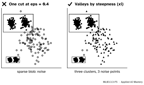
On the blobs of two densities, one fit gives every cut. OPTICS’s own default, the xi method, reads clusters off the steep slopes at the edges of each valley, at whatever depth the valley sits; xi sets how steep a slope must be, and min_cluster_size how wide a valley must be.
from sklearn.datasets import make_blobsXb, yb = make_blobs(n_samples=[100, 100, 100], centers=[(0, 0), (1.2, 0), (4.5, 3)], cluster_std=[0.15, 0.15, 1.5], random_state=1)ob = OPTICS(min_samples=10, xi=0.1, min_cluster_size=30).fit(Xb)for eps in (0.4, 1.0): cut = cluster_optics_dbscan(reachability=ob.reachability_, core_distances=ob.core_distances_, ordering=ob.ordering_, eps=eps)print(f"cut at {eps}: clusters {cut.max() +1}, noise {(cut ==-1).sum()}")table = [[int(((yb == g) & (ob.labels_ == k)).sum()) for k inrange(3)] for g inrange(3)]print("xi clusters:", ob.labels_.max() +1, " noise:", (ob.labels_ ==-1).sum(), " blob by cluster:", table)
cut at 0.4: clusters 2, noise 98
cut at 1.0: clusters 2, noise 10
xi clusters: 3  noise: 3  blob by cluster: [[0, 100, 0], [100, 0, 0], [2, 0, 95]]
The cut at 0.4 leaves 98 points of noise and the cut at 1.0 merges the tight blobs, but the xi method finds the three blobs with only 3 points of noise: each tight blob whole, and 95 of the 100 sparse points together.
Explore
The module’s DBSCAN explorer is in lesson ML03.3.2. Sliding its eps is moving the horizontal line across this lesson’s reachability plot: watch the bridge join cluster 1 as eps passes 2.121, the bar it has here.
Pitfalls
ML03.3.3-F5
Wrong beside right. Cutting the reachability plot with one line repeats DBSCAN’s problem; reading each valley at its own depth keeps all three clusters.
“OPTICS is DBSCAN with a different eps.”
OPTICS on its own clusters nothing; it orders the points. If you then read the plot with one horizontal line, you have run DBSCAN again, with the same single density. The gain comes from reading valleys at different depths, by eye, by the xi method, or with HDBSCAN (next lesson).
“A point’s reachability is a fixed property of the point.”
The core distance is. The reachability is not: it depends on which points were visited before, and so on where the walk started. Only the shape of the plot (its valleys and the bars between them) carries meaning, not the height of one bar taken alone.
“The first bar is infinitely high, so the first point is an outlier.”
The first point has nothing before it, so its reachability is undefined (inf in scikit-learn). Here \((1, 1)\) sits inside cluster 1; the extraction rule judges it by its core distance, 1.414.
Check yourself
Recall
1. Define the core distance of a point when min_samples = m.
Show answer
Its distance to its \((m - 1)\)-th nearest other point: the smallest \(\varepsilon\) at which it is a core point.
2. Give the reachability distance of \(\vect{o}\) from \(\vect{p}\), and say what it means.
Show answer
The larger of the core distance of \(\vect{p}\) and the distance \(d(\vect{p}, \vect{o})\). It is the smallest \(\varepsilon\) at which \(\vect{o}\) is directly density-reachable from \(\vect{p}\).
3. Which point does OPTICS visit next?
Show answer
The unvisited point with the smallest reachability recorded so far (in data order if several tie, and the first unvisited point if all are infinite).
4. On a reachability plot, what is a cluster and what does a horizontal line at \(\varepsilon\) give?
Show answer
A cluster is a valley, a run of low bars. A line at \(\varepsilon\) gives the DBSCAN clustering for that \(\varepsilon\) (up to a few border points): each run below the line is a cluster.
5. In the twelve points, why is the reachability of \((6, 5)\) 2.915 and not its distance 2.121 from the bridge?
Show answer
It is reached from the bridge, whose core distance is 2.915, and the reachability is the larger of that core distance and the distance 2.121.
Exercises
1.★ A core point \(\vect{p}\) has core distance 0.8. Give the reachability from \(\vect{p}\) of points at distances 0.3, 0.8 and 1.7.
Show solution
Take the larger of 0.8 and the distance each time: \(\max(0.8, 0.3) = 0.8\), \(\max(0.8, 0.8) = 0.8\) and \(\max(0.8, 1.7) = 1.7\). The two points inside the core circle are equally easy to reach.
2.★★ Run OPTICS with min_samples = 2 on the six values 1, 2, 4, 8, 11, 12 of lesson ML03.2.1, starting at 1. Give the order and the reachabilities, then read off the clusters for \(\varepsilon' = 2.5\).
Show solution
With \(m = 2\) the core distance is the distance to the nearest other value: 1, 1, 2, 3, 1, 1.
Order 1, 2, 4, 8, 11, 12 with reachabilities \(\infty\), 1, 2, 4, 3, 1.
At \(\varepsilon' = 2.5\): 1 is above but core (1), so it starts cluster 1; 2 and 4 are below and join. 8 is above and not core (3): noise. 11 is above and core (1): it starts cluster 2; 12 is below and joins. Clusters \(\{1, 2, 4\}\) and \(\{11, 12\}\), with 8 as noise.
3.★★★ Show that if a point \(\vect{o}\) is visited with reachability \(r(\vect{o}) \le \varepsilon'\), then it is directly density-reachable at \(\varepsilon'\) from its predecessor, so that it rightly joins the cluster before it.
Show solution
Let \(\vect{p}\) be the predecessor of \(\vect{o}\): the point whose visit set \(r(\vect{o})\). Then
A maximum is at most \(\varepsilon'\) only when both terms are. First, \(\operatorname{core}(\vect{p}) = d_{m-1}(\vect{p}) \le \varepsilon'\), so by the proposition of lesson ML03.3.2, \(\vect{p}\) is a core point at \(\varepsilon'\). Second, \(d(\vect{p}, \vect{o}) \le \varepsilon'\), so \(\vect{o} \in N_{\varepsilon'}(\vect{p})\). These are the two conditions of direct density-reachability. So \(\vect{o}\) belongs to the cluster of the core point \(\vect{p}\), which was visited earlier.
Summary card
Order the points by how easily each is reached; valleys of the plot are clusters at every density.
Reachability of \(\vect{o}\) from \(\vect{p}\): the larger of \(\operatorname{core}(\vect{p})\) and \(d(\vect{p}, \vect{o})\).
Ordering. Visit next the unvisited point of smallest reachability (a priority queue).
Reading. A line at \(\varepsilon\) gives DBSCAN at \(\varepsilon\); the xi method reads valleys at their own depth.
Sources and next steps
Sources. Each was opened and checked against this lesson on 15 November 2026.
Mihael Ankerst, Markus M. Breunig, Hans-Peter Kriegel and Jörg Sander, OPTICS: ordering points to identify the clustering structure, ACM SIGMOD 1999. Section 3.2.1: nested clusters (Figure 3), Definitions 5 and 6 (core-distance, reachability-distance), the seed list ordered by reachability (Figures 5 to 7), and ExtractDBSCAN-Clustering (Figure 8), which may miss some border objects; section 4.1 on reachability plots.
scikit-learn developers, User Guide, section 2.3.9 OPTICS, version 1.9: reachability_ and ordering_, DBSCAN-style extraction with cluster_optics_dbscan for any eps when max_eps is infinite, and the default xi extraction by steep slopes.
Next.ML03.3.4 HDBSCAN builds the same hierarchy of densities as a tree and lets the data choose which clusters to keep.