Carry the kernel estimate into the plane with product kernels and standardised features, draw it as contours over two iris features, see how fast the data needed grow with the dimension, sample new points from an estimate, and build a classifier from one estimate per class.
ML03.8.3L2 Intermediate25 minIn review (what this means)
The maths and code on this page are checked by automated tests on every change, but an independent reader has not signed it off yet. Spot a mistake or a confusing step? Tell us.
Write a product-kernel density estimate in d dimensions, prove it has volume 1, and explain why features are standardised before one bandwidth is shared.
Compute a two-dimensional kernel estimate by hand on the nine points and with KernelDensity.
State the best error rate n to the power minus 4/(4 + d) and explain, with the sample sizes it implies, why kernel estimates fail in many dimensions.
Sample from a kernel estimate by picking a data point and adding kernel noise, and build a Bayes classifier with one kernel estimate per class.
The question
One feature at a time is rarely enough: a flower is its petal length and width, a transaction is its amount and time and place. Can the bump-on-every-point idea describe where data crowd in two, ten or sixty-four dimensions, and what does it cost as the dimension grows?
From the last lesson
1. How does the best bandwidth depend on the sample size \(n\)?
Show answer
It shrinks like \({n^{-1/5}}\): \({h_* = \big(R(\kappa)/(\sigma_\kappa^4 R(f'') n)\big)^{1/5}}\).
2. Why must the likelihood that chooses \(h\) leave each point out?
Show answer
In-sample, each point’s own bump gives it density at least \({\kappa(0)/(nh)}\), which grows without limit as \({h \to 0}\), so the in-sample likelihood always prefers smaller \(h\).
Intuition
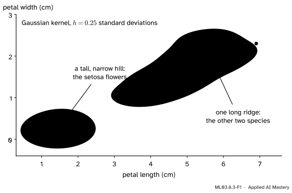
In the plane, a bump is a small hill instead of a small hump: put one on every point and add them, and the sum is a landscape whose height says how crowded the data are nearby. Contour lines, the lines of equal height on a map, draw it.
ML03.8.3-F1
A kernel density estimate of two features of load_iris, drawn as contours. No species labels were used, yet the landscape shows one isolated hill and one long ridge.
The estimate knows nothing about species, yet setosa stands apart as its own hill, while versicolor and virginica merge into one ridge: their petals overlap. A density estimate is a description of where the data are, and that is often the first thing to look at in a new data set. The rest of the lesson asks how wide each hill should be in each direction, and why this simple idea runs out of data so quickly as features are added.
Build it up
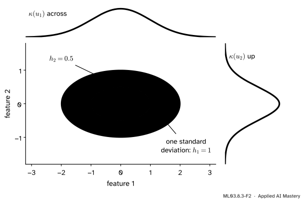
Step 1. One bump per feature, multiplied. The easiest bump in \(d\) dimensions is a product of one-dimensional bumps, one per feature, each with its own bandwidth \({h_j}\). With Gaussian bumps its contours are ellipses lined up with the axes, \({h_1}\) wide across and \({h_2}\) tall up.
ML03.8.3-F2
A product kernel for one point. The hill is the bump across times the bump up, so it can be wider in one feature than in another.
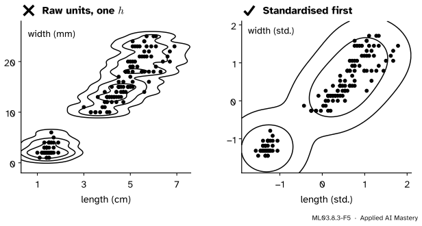
Step 2. Standardise, then share one bandwidth. A bandwidth is a distance in the feature’s own units. If one feature is in centimetres and another in millimetres, the same \(h\) is ten times wider in one than the other. The usual remedy is to divide each feature by its standard deviation first; then one bandwidth, measured in standard deviations, serves every feature. scikit-learn’s KernelDensity takes a single bandwidth, so it expects exactly this.
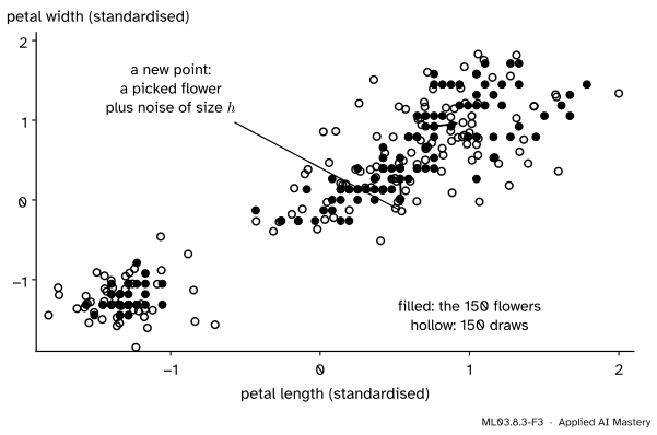
Step 3. Read the estimate as a recipe for new data. In lesson ML03.8.1 the Gaussian estimate was the density of a two-step experiment: pick a data point at random, then add normal noise of size \(h\). Run the experiment and you are sampling from the estimate. Each new point is a real flower, nudged.
ML03.8.3-F3
Sampling from a kernel estimate. Each hollow point is a randomly picked flower plus Gaussian noise with standard deviation \({h = 0.25}\); the draws reproduce the two groups.
The formal statement
NoteDefinition: product-kernel estimate
For data \({\vect{x}_1, \dots, \vect{x}_n}\) in \({\R^d}\) and bandwidths \({h_1, \dots, h_d}\), the product-kernel estimate is
It has volume 1. Each term is a product of functions of one coordinate each, so its integral over \({\R^d}\) is the product of \(d\) one-dimensional integrals. Each of those is 1 by the substitution of lesson ML03.8.1, so each term integrates to 1 and the average of \(n\) such terms to 1.
The Gaussian case. With the Gaussian kernel and one bandwidth \(h\) for every (standardised) feature, the product of the exponentials is the exponential of the sum of squares:
The bump depends only on the distance to the data point, so its contours are circles. This is the estimate that KernelDensity computes.
The curse of dimensionality. The bias of the estimate is still of order \({h^2}\), because the Taylor argument of lesson ML03.8.2 works one coordinate at a time. The variance changes. A bump now has volume of order \({h^d}\), so only about \({n h^d}\) data points fall under it, and the variance is of order \({1/(nh^d)}\). The error therefore behaves like
\[
A\,h^4 + \frac{B}{n h^d}
\]
for constants \(A\) and \(B\) set by \(f\) and \(\kappa\). Minimising over \(h\) (exercise 3) gives \({h \propto n^{-1/(4 + d)}}\) and an error of order
\[
n^{-4/(4 + d)} .
\]
For \({d = 1}\) that is the \({n^{-4/5}}\) of lesson ML03.8.2; for \({d = 10}\) it is \({n^{-2/7}}\), so halving the error takes \({2^{7/2} \approx 11}\) times more data instead of \({2^{5/4} \approx 2.4}\) times. For densities with two smooth derivatives no estimator can beat this rate (Wasserman’s Theorem 6).
ML03.8.3-F6
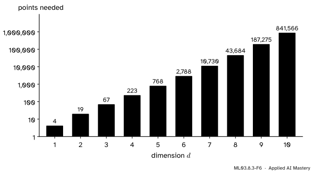
How many points a Gaussian kernel estimate needs, with the best bandwidth, to estimate the standard normal density at its centre with a relative mean squared error below 0.1. Each extra dimension multiplies the requirement by between three and five.
The figure makes the rate concrete. It asks for a modest accuracy, at the easiest possible point, for the nicest possible density, and the answer grows from 4 points in one dimension to 768 in five and 841,566 in ten.
Go deeper: where the numbers in the chart come from
For the standard normal density \(f\) in \({\R^d}\) and the Gaussian kernel, every quantity at \({\vect{0}}\) is a Gaussian integral. The average estimate is the density of a data point plus independent noise, \({N(\vect{0}, (1 + h^2)\mat{I})}\), so \({\E\,\hat f(\vect{0}) = (2\pi(1 + h^2))^{-d/2}}\). One bump at a random data point has second moment
because the exponent is \({-\norm{\vect{x}}^2 (2 + h^2)/(2h^2)}\), a normal density with variance \({h^2/(2 + h^2)}\) up to its constant. The variance of \(\hat f(\vect{0})\) is this minus \({\big(\E\,\hat f(\vect{0})\big)^2}\), divided by \(n\). Add the squared bias, divide by \({f(\vect{0})^2 = (2\pi)^{-d}}\), minimise over \(h\) for each \(n\), and search for the smallest \(n\) that brings the result below 0.1. The code below does exactly that, and checks two of the answers by simulation.
Kernel density classification. With labelled data, fit one estimate \({\hat f_k}\) to the examples of each class \(k\) and take the class shares \({\hat\pi_k}\) as priors. Bayes’ rule (M06.4) gives
and the classifier predicts the class with the largest posterior. Gaussian naive Bayes (ML02.6) is the same recipe with each \({\hat f_k}\) replaced by a product of one bell curve per feature. A kernel estimate can take any shape, so the boundary can bend round curved classes.
ML03.8.3-F7
Two moons: Gaussian naive Bayes draws an almost straight boundary; a kernel estimate per class follows the curved gap. Cross-validated accuracy is 86.5% against 92.25%.
Worked example
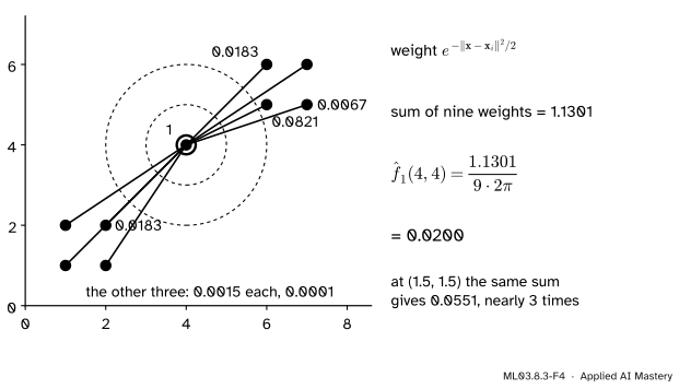
Estimate the density of the nine points at the bridge point \({(4, 4)}\) and at \({(1.5, 1.5)}\), with the Gaussian kernel and \({h = 1}\).
With \({d = 2}\) and \({h = 1}\) the formula is \({\hat f(\vect{x}) = \frac{1}{9 \cdot 2\pi} \sum_i e^{-\norm{\vect{x} - \vect{x}_i}^2/2}}\). Each data point contributes a weight that depends on its squared distance to the query.
At \({(4, 4)}\). The squared distances are 18, 13, 13 and 8 to the lower square (1, 1), (2, 1), (1, 2), (2, 2); 5, 10, 8 and 13 to the upper square (6, 5), (7, 5), (6, 6), (7, 6); and 0 to the bridge point itself. The weights \({e^{-d^2/2}}\), to four decimals, are
and their exact sum is 1.1301 (the rounded terms add to 1.1300). So \(\hat f(4, 4) = {1.1301/(18\pi)} = 0.0200\).
ML03.8.3-F4
The worked example. Only the bridge point itself and the nearest corner (6, 5) matter much; the far square contributes almost nothing.
At \({(1.5, 1.5)}\), the middle of the lower square. Each of the four corners is at squared distance 0.5, weight \({e^{-0.25} = 0.7788}\). The bridge point is at squared distance 12.5, weight 0.0019, and the upper square contributes less than \({10^{-7}}\). The sum is \({4(0.7788) + 0.0019 = 3.1171}\), and
The middle of a cluster is nearly three times as dense as the bridge point, even though the bridge point sits on a data point and the middle of the square does not: four neighbours at distance 0.71 outweigh one at distance 0.
Code
From scratch with the formula above, checked against KernelDensity.
leave-one-out bandwidth: 0.1 distinct flowers: 102 of 150
Leave-one-out picks 0.10, far narrower than the 0.25 of the anchor figure. The reason is in the second number: only 102 of the 150 flowers have distinct petal measurements, because they were measured to a millimetre. A flower with an exact twin is “predicted” perfectly by its twin’s spike, so narrow bandwidths are rewarded. Repeated values fool leave-one-out; the pitfalls return to this.
Next, the chart of the curse of dimensionality, computed from the exact formulas of the .deeper block, and checked by simulation for \({d = 1}\) and \({d = 2}\).
from scipy.optimize import minimize_scalardef relative_mse(n, h, d): f0 = (2* np.pi) ** (-d /2) mean = (2* np.pi * (1+ h * h)) ** (-d /2) second = (2* np.pi * h * h) ** (-d) * (h * h / (2+ h * h)) ** (d /2)return ((mean - f0) **2+ (second - mean **2) / n) / f0 **2def best_h(n, d): r = minimize_scalar(lambda lh: relative_mse(n, np.exp(lh), d), bounds=(-8, 3), method="bounded")return np.exp(r.x), r.fundef points_needed(d): lo, hi =1, 10**8while lo < hi: # binary search for the smallest n that works mid = (lo + hi) //2 lo, hi = (lo, mid) if best_h(mid, d)[1] <0.1else (mid +1, hi)return loneeded = [points_needed(d) for d inrange(1, 11)]print("points needed, d = 1..10:", needed)rng = np.random.default_rng(0)checks = {}for d, n in ((1, needed[0]), (2, needed[1])): h, exact = best_h(n, d) X = rng.normal(size=(100_000, n, d)) # 100,000 samples of size n est = np.exp(-(X **2).sum(axis=2) / (2* h * h)).sum(axis=1) / (n * (2* np.pi * h * h) ** (d /2)) f0 = (2* np.pi) ** (-d /2) checks[d] = (exact, np.mean((est - f0) **2) / f0 **2)print(f"d = {d}, n = {n}, h = {h:.3f}: exact {exact:.4f}, simulated {checks[d][1]:.4f}")
points needed, d = 1..10: [4, 19, 67, 223, 768, 2788, 10730, 43684, 187275, 841566]
d = 1, n = 4, h = 0.781: exact 0.0877, simulated 0.0880
d = 2, n = 19, h = 0.534: exact 0.0981, simulated 0.0975
Sampling, from scratch and with KernelDensity.sample. Both draws should have the data’s mean, and each feature’s variance should be the data’s (1, after standardising) plus \({h^2}\), because the noise adds its own variance.
h =0.25picks = rng.integers(0, len(Z), size=20_000)ours = Z[picks] + h * rng.normal(size=(20_000, 2)) # pick a flower, add kernel noisetheirs = KernelDensity(bandwidth=h).fit(Z).sample(20_000, random_state=0)print("means:", ours.mean(axis=0).round(2) +0.0, theirs.mean(axis=0).round(2) +0.0) # + 0.0 turns -0.0 into 0.0print("variances:", ours.var(axis=0).round(3), theirs.var(axis=0).round(3), " expected", 1+ h * h)
KernelDensity also speeds up evaluation with a tree. Points far from a query add almost nothing, and a k-d tree or ball tree groups nearby points, so whole groups can be judged at once; rtol allows a small relative error in exchange for more pruning.
On the iris petals, where each species is a compact blob, the two tie at 96%. On the moons, where each class is curved, the kernel estimates win, 92.25% against 86.5%.
Explore
This module’s interactive, the bandwidth explorer, lives in ML03.8.2. It works on a line, but everything you see there carries over: in two dimensions each dot gets a small hill instead of a bump, and the bandwidth slider sets the hills’ width in every direction at once.
Pitfalls
ML03.8.3-F5
Wrong beside right. With petal width in millimetres, a bandwidth of 0.5 is far too narrow up and the contours turn ragged around single rows of flowers. After standardising, the same bandwidth fits both features.
“One bandwidth is fine; the features are all just numbers.”
A bandwidth is a distance, so it has units. Measure petal width in millimetres instead of centimetres and the same \(h\) becomes ten times narrower in that direction. Standardise first, or give each feature its own bandwidth.
“Leave-one-out always finds a sensible bandwidth.”
Not when values repeat. On the iris petals there are only 102 distinct pairs of measurements, so 48 flowers repeat a pair already in the data. Each twin predicts the other perfectly with a narrow spike, and leave-one-out picks 0.10. Rounded or repeated data need \(k\)-fold cross-validation with larger folds, a little added jitter, or simply judgement.
“With enough data a kernel estimate works in any dimension.”
“Enough” grows exponentially: 768 points for a rough estimate at the centre of a five-dimensional normal, 841,566 in ten. On images or text, first reduce the dimension (the scikit-learn digits example projects 64 pixels to 15 principal components before fitting KernelDensity), or use a model with fewer parameters, such as a Gaussian mixture.
Check yourself
Recall
1. Write the Gaussian kernel estimate in \({\R^d}\) with one bandwidth \(h\).
2. Why standardise features before using a single bandwidth?
Show answer
A bandwidth is a distance in each feature’s units; after standardising, every feature is measured in standard deviations, so one \(h\) means the same width in every direction.
3. What is the best error rate of a kernel estimate in \(d\) dimensions, and why is it slower than in one?
Show answer
\({n^{-4/(4 + d)}}\). The bias is still of order \({h^2}\), but a bump of width \(h\) covers a volume of order \({h^d}\), so the variance is of order \({1/(nh^d)}\).
4. How do you sample from a Gaussian kernel estimate?
Show answer
Pick one of the \(n\) data points uniformly at random and add Gaussian noise with standard deviation \(h\) in every coordinate.
5. How does a kernel density classifier predict, and how does it differ from Gaussian naive Bayes?
Show answer
It fits one estimate \({\hat f_k}\) per class and predicts the class with the largest \({\hat\pi_k \hat f_k(\vect{x})}\). Naive Bayes uses a product of one normal curve per feature instead, so it cannot follow curved or multi-humped classes.
Exercises
1.★ Estimate the density of the nine points at \({(6.5, 5.5)}\), the middle of the upper square, with the Gaussian kernel and \({h = 1}\).
Show solution
The four upper corners are at squared distance 0.5, each with weight \({e^{-0.25} = 0.7788}\). The bridge point is at squared distance \({2.5^2 + 1.5^2 = 8.5}\), weight \({e^{-4.25} = 0.0143}\). The lower square is at squared distance 32.5 or more and adds nothing visible. The sum is \({3.1152 + 0.0143 = 3.1295}\), so \(\hat f(6.5, 5.5) = {3.1295/(18\pi)} = 0.0553\), slightly above the lower square’s 0.0551 because the bridge point is a little nearer.
2.★★ If the error falls like \({n^{-4/(4 + d)}}\), by what factor must \(n\) grow to halve the error in \({d = 1}\) and in \({d = 6}\)?
At \({h_*}\), the first term is \({A h_*^4 \propto n^{-4/(d + 4)}}\). For the second, the condition gives \({B/(nh_*^d) = \tfrac{4A}{d} h_*^4}\), the same power of \(n\). So \({E(h_*) = A h_*^4 (1 + 4/d) \propto n^{-4/(d + 4)}}\). The second derivative is positive, so this is a minimum.
Summary card
In \(d\) dimensions, bumps become hills, and the data needed explode.
ML03.8.3-F1
Iris petals, one hill and one ridge.
Product kernel: one bump per feature, multiplied; standardise the features and share one \(h\).
Curse: error \({\propto n^{-4/(4 + d)}}\); 4 points in one dimension, 841,566 in ten for the same accuracy.
Sampling: pick a data point, add kernel noise; KernelDensity.sample.
Classifier:\({\arg\max_k \hat\pi_k \hat f_k(\vect{x})}\), one estimate per class.
Sources and next steps
Sources. Each was opened and checked against this lesson on 15 November 2026.
T. Hastie, R. Tibshirani and J. Friedman, The Elements of Statistical Learning, 2nd edition, corrected 12th printing. Section 6.6.1: the Gaussian product kernel in \({\R^p}\) (equation 6.24) and the estimate as Gaussian noise added to each observation (6.23); Section 6.6.2: kernel density classification by Bayes’ theorem (6.25), and the warning that the estimates are of poor quality where data are sparse.
L. Wasserman, Density Estimation, lecture notes for 36-708, Carnegie Mellon University. Section 4.1, Theorem 5: risk of order \({h^4 + 1/(nh^d)}\) and, with \({h \asymp n^{-1/(4 + d)}}\), the rate \({n^{-4/(4 + d)}}\); Theorem 6 and the remark that kernel estimators are rate minimax; Section 6 on why the rate is hopeless in high dimensions.
scikit-learn, KernelDensity: one bandwidth, algorithm'kd_tree' or 'ball_tree', tolerances atol and rtol (“a larger tolerance will generally lead to faster execution”), and sample, implemented for the Gaussian and tophat kernels only; and the example Kernel Density Estimation, which reduces the digits to 15 principal components before fitting and sampling.
Next.ML03.8.4 Mean shift climbs the hills of a kernel estimate to find clusters, and ML03.9 uses low density as a score of strangeness.