A small bandwidth follows the noise and a large one smooths away the shape. Derive the bias and variance behind that trade-off, the best bandwidth shrinking like n to the minus one fifth, the rules of thumb of Silverman, and leave-one-out likelihood as a choice made by the data.
ML03.8.2L2 Intermediate25 minIn review (what this means)
The maths and code on this page are checked by automated tests on every change, but an independent reader has not signed it off yet. Spot a mistake or a confusing step? Tell us.
Derive the bias of order h squared times f’’ and the variance of order f/(nh) of a kernel estimate by Taylor expansion.
Minimise the asymptotic mean integrated squared error to show that the best bandwidth shrinks like n to the power minus one fifth.
Compute the normal reference rule and Silverman’s rule of thumb, and say when they smooth too much.
Choose a bandwidth by leave-one-out log-likelihood, from scratch and with GridSearchCV, and compare density estimates by held-out log-likelihood.
The question
Every kernel estimate needs a bandwidth \(h\), and the picture changes completely with it: tiny \(h\) gives a spike on every point, huge \(h\) gives one featureless hump. Is there a best \(h\), how does it depend on the amount of data, and how can we find it when the true density is exactly what we do not know?
From the last lesson
1. Write the kernel density estimate with kernel \(\kappa\) and bandwidth \(h\).
2. Why does a histogram’s picture change when its bins move, while a kernel estimate’s does not?
Show answer
A histogram counts points in fixed bins, so the counts depend on where the bins start. A kernel estimate centres a bump on every point, so there is no origin to choose.
Intuition
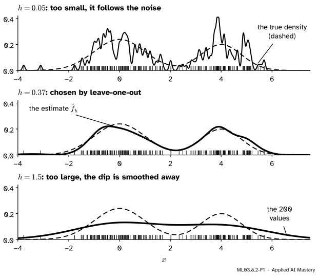
Draw 200 values from a known two-humped density, \({0.6\,N(0, 1) + 0.4\,N(4, 0.8^2)}\), and estimate it with three bandwidths.
ML03.8.2-F1
The same 200 values, three bandwidths. The estimate against the true density (dashed). Too small a bandwidth shows noise as structure; too large hides real structure.
With \({h = 0.05}\) each bump is narrower than the gaps between neighbouring values, so the estimate is a comb of spikes. Draw another 200 values and the spikes would all move: the estimate has high variance. With \({h = 1.5}\) each bump is wider than the dip between the humps, so the dip is filled in. Draw another sample and you get almost the same plateau, but it is systematically wrong: the estimate has high bias. The middle bandwidth balances the two. The rest of the lesson makes this balance exact and then lets the data strike it.
Build it up
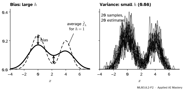
Step 1. The average estimate is a blurred truth. Imagine drawing many samples of size \(n\) and averaging their estimates. Each term of the estimate has the same average, so the average estimate is the true density seen through the kernel: every value of \(f\) is replaced by a kernel-weighted average of \(f\) around it. A blur lowers peaks and fills dips. That gap between the blurred truth and the truth is the bias, and it grows with \(h\).
Step 2. One sample’s estimate wobbles around that average. With a small \(h\), the estimate at \(x\) depends on the few values that happen to fall within about \(h\) of \(x\). Few values mean a noisy count, so the estimate wobbles from sample to sample. That wobble is the variance, and it shrinks as \(h\) or \(n\) grows.
ML03.8.2-F2
Left: the average estimate for \({h = 1}\) is the truth blurred, so it misses low at peaks and high in dips. Right: with \({h = 0.08}\), estimates from 20 different samples disagree wildly.
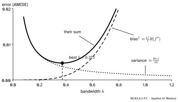
Step 3. Add the two errors. The mean squared error at \(x\) is bias squared plus variance. Bias squared rises with \(h\), variance falls with \(h\), so their sum has a lowest point. Adding the error over all \(x\) gives one number per \(h\), and the best \(h\) minimises it.
The formal statement
Write \({\sigma_\kappa^2 = \int u^2 \kappa(u)\,du}\) for the kernel’s variance and \({R(g) = \int g(x)^2\,dx}\) for the “roughness” of a function. The mean integrated squared error is \({\mathrm{MISE}(h) = \E \int \big(\hat f_h(x) - f(x)\big)^2 dx}\), the expected squared gap between estimate and truth, added over all \(x\).
The bias. The estimate is the mean of \(n\) independent copies of \({\tfrac1h \kappa\big((x - X)/h\big)}\), so its expectation is that of one copy:
Integrate each term against \(\kappa\). The first gives \({f(x)}\) because \({\int\kappa = 1}\); the second gives 0 because \({\int u\,\kappa(u)\,du = 0}\) for a symmetric kernel; the third gives \({\tfrac12 h^2 \sigma_\kappa^2 f''(x)}\). So
Where \(f\) curves down (a peak, \({f'' < 0}\)) the estimate is too low; where it curves up (a dip) it is too high. That is the left panel above.
The variance. Call one copy \({Y = \tfrac1h \kappa\big((x - X)/h\big)}\). The variance of a mean of \(n\) independent copies is \({1/n}\) times the variance of one copy, and a variance is at most the second moment, so \({\mathrm{Var}\,\hat f_h(x) \le \E[Y^2]/n}\). The second moment is
so \({\mathrm{Var}\,\hat f_h(x) \approx f(x)R(\kappa)/(nh)}\). The second line is the same substitution, which leaves one factor \({1/h}\) over, and the third keeps only the first Taylor term \({f(x)}\). The part we dropped, the squared mean \({\big(\E\,\hat f_h(x)\big)^2 / n}\), is of order \({1/n}\) and so is small next to \({1/(nh)}\) when \(h\) is small: the bound is the leading term.
The best bandwidth. Squaring the bias, adding the variance and integrating over \(x\) (where \({\int f = 1}\)) gives the asymptotic MISE:
The best bandwidth shrinks like \({n^{-1/5}}\): a thousand times more data allows bumps only about four times narrower (\({1000^{1/5} = 3.98}\)). Put \({h_*}\) back and both terms are of order \({n^{-4/5}}\), slower than the \({1/n}\) of a model with a fixed number of parameters.
ML03.8.2-F3
The two terms of AMISE for the two-humped density and \({n = 200}\). Their sum is lowest at \({h_* = 0.373}\).
Rules of thumb.\({h_*}\) needs \({R(f'')}\), which depends on the unknown \(f\). If we pretend \(f\) is normal with standard deviation \(\sigma\) and use the Gaussian kernel (\({\sigma_\kappa^2 = 1}\), \({R(\kappa) = 1/(2\sqrt\pi)}\)), then \({R(f'') = 3/(8\sqrt\pi\,\sigma^5)}\) and
the normal reference rule, with \(\sigma\) estimated from the data. This lesson uses the sample standard deviation \(s\); Wasserman’s notes use the smaller of \(s\) and \({\mathrm{IQR}/1.34}\), which gives the same value in both examples below. Silverman’s rule of thumb uses a smaller factor and a spread that resists outliers:
\[
h = 0.9\, \min\!\left(s, \frac{\mathrm{IQR}}{1.34}\right) n^{-1/5} ,
\]
where \(s\) is the sample standard deviation and IQR the interquartile range (for normal data \({\mathrm{IQR} \approx 1.34\,\sigma}\), so both measure \(\sigma\)). Both rules are tuned for one bell; on data with several humps they smooth too much.
Go deeper: the roughness of a normal density's second derivative
For \({f = N(0, \sigma^2)}\) write \({z = x/\sigma}\). Then \({f''(x) = f(x)\,(z^2 - 1)/\sigma^2}\) and \({f(x)^2 = e^{-z^2}/(2\pi\sigma^2)}\), so with \({dx = \sigma\,dz}\)
\[
R(f'') = \frac{I}{2\pi\sigma^5} ,
\]
where
\[
I = \int (z^4 - 2z^2 + 1)\, e^{-z^2}\,dz .
\]
The three Gaussian integrals are \({\int z^4 e^{-z^2} dz = \tfrac34\sqrt\pi}\), \({\int z^2 e^{-z^2} dz = \tfrac12\sqrt\pi}\) and \({\int e^{-z^2} dz = \sqrt\pi}\), so the bracket integrates to \(I = {\sqrt\pi\,(\tfrac34 - 1 + 1)} = {\tfrac34\sqrt\pi}\) and \({R(f'') = 3/(8\sqrt\pi\,\sigma^5)}\). Dividing \({R(\kappa) = 1/(2\sqrt\pi)}\) by it gives \({\tfrac{8\sigma^5}{6} = \tfrac43\sigma^5}\), whose fifth root is the rule.
Letting the data choose: leave-one-out likelihood. A good estimate should give high density to new values from the same source. We have no new values, but we can pretend: leave \(x_i\) out, build the estimate from the other \({n - 1}\), and score \(x_i\) by it:
The leave-one-out log-likelihood\(\mathrm{CV}(h)\) is the average log density that held-out points receive. Choose the \(h\) that maximises it. On the two humps it picks \({h = 0.37}\), the middle panel of the anchor figure, almost exactly the \({h_* = 0.373}\) that AMISE gives with the true density in hand.
Worked example
Choose a bandwidth for the six values 1, 2, 3, 6, 8 and 9.
Rules of thumb. The mean is \({29/6 = 4.833}\) and the squared deviations sum to 54.833, so \({s = \sqrt{54.833/5} = 3.312}\). NumPy’s quartiles are 2.25 and 7.5, so \({\mathrm{IQR} = 5.25}\) and \({\mathrm{IQR}/1.34 = 3.918}\). The smaller of \(s\) and 3.918 is \(s\). With \({n^{-1/5} = 6^{-0.2} = 0.6988}\), the normal reference rule \({h_{\text{NR}}}\) and Silverman’s rule \({h_{\text{S}}}\) give
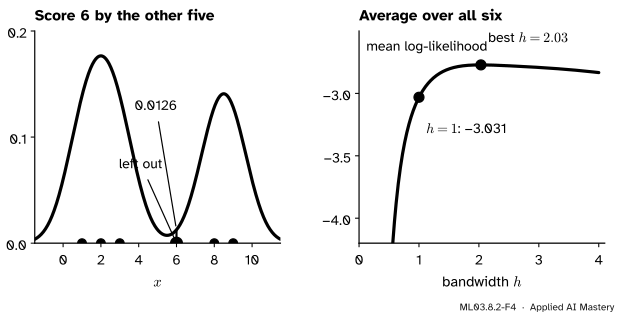
Leave-one-out at \({h = 1}\). Leave out 6 and build the estimate from the other five values. The distances from 6 to them are 5, 4, 3, 2 and 3. Write \({S_{-4}(6)}\) for the sum of their five kernel values; then
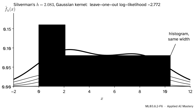
The worked example. Left: leaving 6 out, the other five give it density 0.0126. Right: averaging the six log scores for every \(h\) traces \(\mathrm{CV}(h)\), highest at \({h = 2.03}\).
Doing the same for every value gives densities 0.0592, 0.0968, 0.0601, 0.0126, 0.0592 and 0.0493, whose logs average to \({\mathrm{CV}(1) = -3.031}\). The value 6 costs most: \({\ln 0.0126 = -4.374}\). A wider bandwidth lets the neighbours reach it. Repeating for a grid of \(h\) gives the curve on the right; its maximum is \({-2.772}\) at \({h = 2.03}\), close to Silverman’s 2.083. With only six values the data cannot support fine detail, and all three choices are wide.
Code
Leave-one-out from scratch: one \({n \times n}\) matrix of kernel values, with the diagonal set to zero so that no point scores itself.
import numpy as npdef loo_loglik(data, h): u = (data[:, None] - data[None, :]) / h k = np.exp(-u **2/2) / np.sqrt(2* np.pi) np.fill_diagonal(k, 0.0) # leave each point out of its own estimatereturn np.mean(np.log(k.sum(axis=1) / ((len(data) -1) * h)))x = np.array([1, 2, 3, 6, 8, 9], dtype=float)n =len(x)s = x.std(ddof=1)q1, q3 = np.percentile(x, [25, 75])normal_ref =1.06* s * n **-0.2silverman =0.9*min(s, (q3 - q1) /1.34) * n **-0.2grid = np.round(np.arange(0.5, 4.001, 0.01), 2)cv = np.array([loo_loglik(x, h) for h in grid])best = grid[cv.argmax()]print(f"s = {s:.3f}, IQR = {q3 - q1}, normal reference {normal_ref:.3f}, Silverman {silverman:.3f}")print(f"CV(1) = {loo_loglik(x, 1.0):.3f}; best h on the grid = {best}, CV = {cv.max():.3f}")
s = 3.312, IQR = 5.25, normal reference 2.453, Silverman 2.083
CV(1) = -3.031; best h on the grid = 2.03, CV = -2.772
scikit-learn does the same search with GridSearchCV. KernelDensity.score returns the total log-likelihood of the data it is given, so with LeaveOneOut each fold scores one held-out value, and the best mean score is our \(\mathrm{CV}(h)\).
Now the two humps, with a test set of 2000 values from the same density. We compare a kernel estimate with leave-one-out \(h\), the two rules of thumb, a two-component Gaussian mixture fitted by EM (ML03.4) and a histogram, all by their mean log density on the test values.
from scipy.stats import normfrom sklearn.mixture import GaussianMixturerng = np.random.default_rng(0)def two_humps(m): first = rng.random(m) <0.6return np.where(first, rng.normal(0, 1, m), rng.normal(4, 0.8, m))train, test = two_humps(200), two_humps(2000)hs = np.round(np.arange(0.05, 1.501, 0.01), 2)h_loo = hs[np.argmax([loo_loglik(train, h) for h in hs])]s2 = train.std(ddof=1)q1, q3 = np.percentile(train, [25, 75])rules = {"leave-one-out": h_loo, "Silverman": 0.9*min(s2, (q3 - q1) /1.34) *200**-0.2,"normal reference": 1.06* s2 *200**-0.2}scores = {}for name, h in rules.items(): scores[name] = KernelDensity(bandwidth=h).fit(train[:, None]).score_samples(test[:, None]).mean()print(f"kernel estimate, {name:16s} h = {h:.3f}: {scores[name]:.4f}")mix = GaussianMixture(n_components=2, random_state=0).fit(train[:, None])truth = np.log(0.6* norm.pdf(test) +0.4* norm.pdf(test, 4, 0.8)).mean()edges = np.arange(-5, 9.001, 0.5)counts, _ = np.histogram(train, edges)hist_at_test = (counts / (200*0.5))[np.searchsorted(edges, test, side="right") -1]print(f"Gaussian mixture, K = 2: {mix.score(test[:, None]):.4f}; true density: {truth:.4f}")print("histogram, width 0.5: test values in empty bins:", int(np.sum(hist_at_test ==0)))five_fold = GridSearchCV(KernelDensity(), {"bandwidth": hs}).fit(train[:, None]).best_params_["bandwidth"]print("5-fold GridSearchCV picks h =", five_fold)
kernel estimate, leave-one-out    h = 0.370: -1.9758
kernel estimate, Silverman        h = 0.699: -1.9977
kernel estimate, normal reference h = 0.823: -2.0198
Gaussian mixture, K = 2: -1.9625;  true density: -1.9523
histogram, width 0.5: test values in empty bins: 27
5-fold GridSearchCV picks h = 0.39
The ranking is honest. The mixture wins, at \({-1.963}\) against the truth’s \({-1.952}\), because the data really are a mixture of two normals: the right parametric model is hard to beat. The kernel estimate with the leave-one-out bandwidth comes close at \({-1.976}\) without assuming any shape. Both rules of thumb smooth too much (0.699 and 0.823 against 0.37) and score lower. The histogram scores \({-\infty}\): 27 test values land in bins that held no training value, where it says the density is exactly 0. Five-fold GridSearchCV, the default, picks 0.39, close to leave-one-out.
Explore
ML03.8-X1
Bandwidth explorer
Drag the points along the line, or pick one with the buttons and move it with its slider. Slide the bandwidth, switch the kernel, and press the buttons for Silverman’s rule and for the leave-one-out best. Switch on the histogram to compare it with bins of the same width.
Three things to try. Make \(h\) small and watch the leave-one-out score fall as the spikes stop reaching their neighbours. Choose the tophat kernel with \({h = 1}\): the score is \({-\infty}\), because 6 has no other point within 1. Then drag one point far to the right and press Silverman again: the outlier inflates \(s\), but the IQR, and so the rule, barely moves.
Pitfalls
ML03.8.2-F5
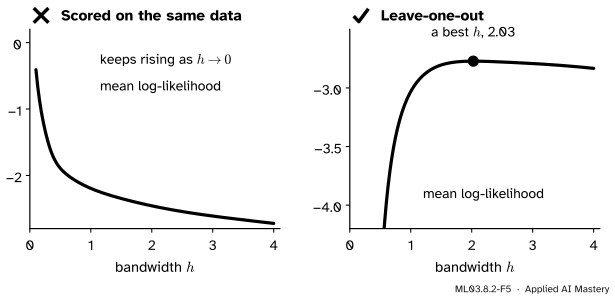
Wrong beside right. Scored on its own data, the likelihood always prefers a smaller bandwidth. Leaving each point out gives a curve with a real maximum.
“Pick the bandwidth that maximises the likelihood of the data.”
Not of the same data. At each data point the estimate is at least the point’s own bump, \({\kappa(0)/(nh)}\), which grows without limit as \({h \to 0}\). So the in-sample likelihood rewards ever narrower spikes. Only held-out points, by leaving one out or by \(k\)-fold cross-validation, can say when the spikes have stopped helping.
“Silverman’s rule is a safe default.”
It is safe for one bell. On the two humps it gives 0.699, nearly twice the leave-one-out 0.37, and a worse held-out score. On the six values the normal reference rule gives 2.453, wide enough to merge the two groups into a single hill (lesson ML03.8.4 counts the hills). Use a rule for a first look and cross-validation for a decision.
“A bandwidth of 1 means the same in every library.”
KernelDensity(bandwidth=1) uses Gaussian bumps of standard deviation 1. gaussian_kde(x, bw_method=1) uses bumps whose standard deviation is 1 times the sample’s, here 3.312. And MeanShift(bandwidth=1) in lesson ML03.8.4 uses a flat window of radius 1. Read the documentation before copying a number.
Check yourself
Recall
1. What are the leading bias and variance of a kernel estimate at \(x\)?
4. Why must the likelihood used to choose \(h\) leave each point out?
Show answer
Because a point’s own bump gives it density at least \({\kappa(0)/(nh)}\), so the in-sample likelihood grows without limit as \({h \to 0}\).
5. On the two humps, which estimate had the best held-out score, and why did the histogram score \({-\infty}\)?
Show answer
The two-component Gaussian mixture, because the data really are such a mixture. The histogram gave density 0 to 27 test values that fell in bins with no training value, and \({\ln 0 = -\infty}\).
Exercises
1.★ Ten more values are added to the six, making \({n = 16}\), and the spread \(s\) stays at 3.312 with \({\mathrm{IQR}/1.34}\) still larger. What does Silverman’s rule give now?
Show solution
\(16^{-0.2} = e^{-0.2 \ln 16} = e^{-0.5545} = 0.5743\), so \(h = {0.9 \cdot 3.312 \cdot 0.5743} = 1.712\). Nearly three times as many values shrink the bandwidth by the factor \({(16/6)^{-1/5} = 0.822}\) only.
2.★★ With the tophat kernel and \({h = 1}\), show that the leave-one-out log-likelihood of the six values is \({-\infty}\). How large must \(h\) be before it is finite?
Show solution
The tophat estimate at \(x_i\) without \(x_i\) counts the other points within \(h\). The value 6 has its nearest neighbour, 8, at distance 2, so with \({h = 1}\) its leave-one-out density is 0 and its log is \({-\infty}\); one infinite term makes the average \({-\infty}\). Every other value has a neighbour 1 away. The score is finite once every point has a neighbour inside its window. The largest nearest-neighbour distance is 2, so with the window \({\abs{u} \le 1}\) of lesson ML03.8.1 the score is finite from \({h = 2}\) on; scikit-learn, which leaves a point exactly \(h\) away outside, needs \(h\) above 2.
3.★★★ For the Epanechnikov kernel, compute \({R(\kappa)}\) and \({\sigma_\kappa^2}\), and derive its normal reference bandwidth.
so \(h_* = {(40\sqrt\pi)^{1/5}\,\sigma n^{-1/5}} = {2.345\,\sigma n^{-1/5}}\). It is larger than the Gaussian’s 1.06 because the Epanechnikov kernel’s own standard deviation is only \({1/\sqrt5}\); in those units, \({2.345/\sqrt5 = 1.049}\), almost the same smoothing.
Summary card
Bandwidth trades bias against variance; let held-out likelihood choose it.
ML03.8.2-F1
Too small, about right, too large.
Bias: about \({\tfrac12 h^2\sigma_\kappa^2 f''(x)}\).
Variance: about \({f(x)R(\kappa)/(nh)}\).
Best \(h\): shrinks like \({n^{-1/5}}\); the error then falls like \({n^{-4/5}}\).
Rules:\({1.06\,s\,n^{-1/5}}\); Silverman uses 0.9 and the smaller of \(s\) and \({\mathrm{IQR}/1.34}\).
Data-driven: maximise the leave-one-out log-likelihood, or use GridSearchCV with KernelDensity.
Sources and next steps
Sources. Each was opened and checked against this lesson on 15 November 2026.
L. Wasserman, Density Estimation, lecture notes for 36-708, Carnegie Mellon University. Section 5.3, Theorem 14: the bias \({\tfrac12\sigma_K^2 h^2 p''(x)}\) and variance \({p(x)\int K^2/(nh)}\) derived by the substitution and Taylor expansion used here, the integrated risk (31) and the best bandwidth (32), decreasing at rate \({n^{-1/5}}\) with risk \({O(n^{-4/5})}\). Section 15: the normal reference rule \({1.06\,\sigma n^{-1/5}}\) with \(\sigma\) estimated by \({\min\{s, Q/1.34\}}\), and the advice to prefer cross-validation.
statsmodels, bw_silverman: returns \({0.9\,A\,n^{-1/5}}\), where \(A\) is the smaller of the standard deviation (with \({n - 1}\)) and \({\mathrm{IQR}/1.349}\), citing B. W. Silverman, Density Estimation for Statistics and Data Analysis (Chapman and Hall, 1986).
scikit-learn, Density Estimation, User Guide Section 2.8.2: the bandwidth “controls the tradeoff between bias and variance”; and the example Kernel Density Estimation, which chooses the bandwidth of KernelDensity with GridSearchCV.