Turn a sample into a smooth curve of area 1 by putting a small bump on every point and adding the bumps. See why histograms depend on where the bins start, prove that a kernel estimate has area 1, and compute one by hand, from scratch and with SciPy and scikit-learn.
ML03.8.1L2 Intermediate25 minIn review (what this means)
The maths and code on this page are checked by automated tests on every change, but an independent reader has not signed it off yet. Spot a mistake or a confusing step? Tell us.
Explain the two faults of a histogram as a density estimate: it depends on where the bins start, and it is a staircase.
Write the kernel density estimate with bandwidth h and kernel kappa, and name the Gaussian, Epanechnikov and tophat kernels.
Prove that a kernel density estimate is never negative and has area 1.
Compute a kernel density estimate by hand at a few points and match it with NumPy, scipy.stats.gaussian_kde and sklearn.neighbors.KernelDensity.
The question
You have six numbers, 1, 2, 3, 6, 8 and 9, and you want the curve they were drawn from: high where values crowd, low where they are rare, with area 1 like every density. A histogram is the usual answer, but slide its bins by one unit and the picture changes. Is there an estimate that does not depend on such an arbitrary choice, and that is smooth enough to use in a model?
Intuition
A density estimate turns a sample \({x_1, \dots, x_n}\) into a curve \(\hat f\) with area 1. Its height says how crowded the data are near each \(x\). Machine learning uses such curves everywhere: to score how strange a new value is (anomaly detection, ML03.9), to classify by Bayes’ rule, to draw new data that look like the old, and to find clusters as the hills of the curve (lesson ML03.8.4).
The idea of this lesson fits in one sentence: put a small bump of area \({1/n}\) on every data point, and add the bumps.
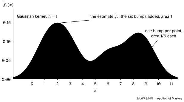
ML03.8.1-F1
A kernel density estimate of the six values. Each point spreads into a bump of area \({1/6}\); their sum is the estimate. Where bumps overlap, the estimate is high.
Where three points sit close together (1, 2 and 3) their bumps pile up into a tall hill. Where there is a gap (between 3 and 6) only the tails of bumps reach, and the curve dips. Nothing about the picture depends on where a bin starts, because there are no bins. The width of the bumps, the bandwidth\(h\), is the one choice left, and lesson ML03.8.2 is about choosing it.
Build it up
Step 1. The histogram as a density estimate. In S01.4.1 you made a histogram on the density scale: cut the line into bins of width \(h\), count the values \(n_j\) in each bin, and draw a bar of height \({n_j / (nh)}\). The area of a bar is \({n_j / n}\), its share of the data, so the bars have total area 1. That is already a density estimate. It has two faults.
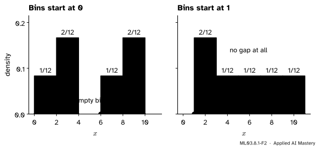
ML03.8.1-F2
The same six values and the same bin width 2. Starting the bins at 0 shows two groups with a gap; starting them at 1 hides the gap completely. Heights are density, count over \({nh = 12}\).
Fault 1: it depends on the bin origin. Nothing in the data says where bins should start, yet the answer to “is there a gap between the groups?” changes when they move. Fault 2: it is a staircase. The estimate jumps at every bin edge and is flat in between, so its slope is zero or undefined everywhere. A model that needs a slope, such as the hill climbing of ML03.8.4, cannot use it.
Step 2. Centre the bin on the point you ask about. To estimate the density at \(x\), count the values within \(h\) of \(x\) and divide by \({n \cdot 2h}\), the sample size times the window’s width. This moving window has no origin to choose: the window moves with \(x\). Read the other way round, each data point contributes \({1/(2nh)}\) to every \(x\) within \(h\) of it. So the moving window is a sum of small boxes, one centred on each point, each of width \(2h\) and area \({1/n}\). That box is the first kernel.
Step 3. Use a smooth bump instead of a box. The boxes still have edges, so the sum still jumps. Replace each box with a bump that rises and falls smoothly, such as a bell curve, and the sum is smooth too. The shape of one bump is called the kernel.
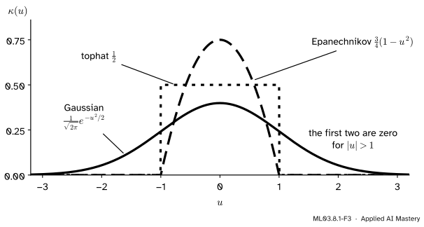
ML03.8.1-F3
The three kernels of this lesson. Each is a density of area 1 centred on 0. The tophat and Epanechnikov kernels vanish outside \({[-1, 1]}\); the Gaussian has tails that go on for ever.
The formal statement
NoteDefinition: kernel density estimate
A kernel is a function \({\kappa(u) \ge 0}\) with \({\int \kappa(u)\,du = 1}\) that is symmetric, \({\kappa(-u) = \kappa(u)}\). Given a sample \({x_1, \dots, x_n}\) and a bandwidth\({h > 0}\), the kernel density estimate is
where the last two hold for \({\abs{u} \le 1}\) and are 0 outside. The Gaussian kernel is the standard normal density, so with it each bump is a normal density with mean \(x_i\) and standard deviation \(h\).
Reading the formula. The fraction \({(x - x_i)/h}\) measures how far \(x\) is from the data point, in units of \(h\). The kernel turns that distance into a weight that is largest when \(x\) sits on the point. Summing over \(i\) adds the bumps, and the factor \({1/(nh)}\) scales them so that the total area is 1.
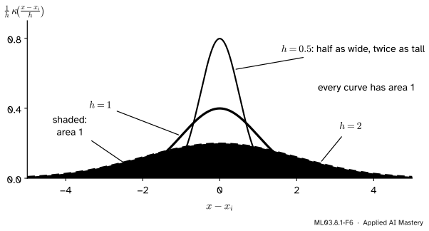
ML03.8.1-F6
One bump, \({\tfrac1h \kappa\big((x - x_i)/h\big)}\), for three bandwidths. Dividing by \(h\) exactly undoes the stretch, so the area stays 1 whatever \(h\) is.
The estimate is a density. Two things must hold. First, \({\hat f_h(x) \ge 0}\), because every kernel value is at least 0 and \({nh > 0}\). Second, the area is 1. Integrate the sum term by term:
In the \(i\)-th integral substitute \({u = (x - x_i)/h}\). Then \({x = x_i + hu}\), so \({dx = h\,du}\), and as \(x\) runs over the whole line so does \(u\). The integral becomes
Each of the \(n\) terms is 1, so the total is \({\tfrac1n \cdot n = 1}\). The figure above is this substitution as a picture: stretching by \(h\) multiplies the area by \(h\), and the factor \({1/h}\) divides it back.
Another way to see it. With the Gaussian kernel, the estimate is exactly the density of this two-step experiment: pick one of the \(n\) data points at random, then add normal noise with standard deviation \(h\). Hastie, Tibshirani and Friedman describe the estimate this way, as the sample smoothed by adding independent Gaussian noise to each observation. Lesson ML03.8.3 turns the experiment into a way to sample new data.
Worked example
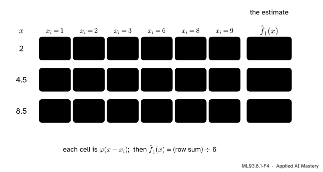
Estimate the density of the six values at \({x = 2}\), \({x = 4.5}\) and \({x = 8.5}\), with the Gaussian kernel and \({h = 1}\).
With \({h = 1}\) the formula is \({\hat f_1(x) = \tfrac16 \sum_i \varphi(x - x_i)}\), where \({\varphi(u) = e^{-u^2/2}/\sqrt{2\pi}}\) is the Gaussian kernel. Its values at the distances that occur are \({\varphi(0) = 0.3989}\), \({\varphi(0.5) = 0.3521}\), \({\varphi(1) = 0.2420}\), \({\varphi(1.5) = 0.1295}\) and \({\varphi(2.5) = 0.0175}\); beyond a distance of 3 they are below 0.005. Write \({S(x)}\) for the sum of the six kernel values at \(x\), so that \({\hat f_1(x) = S(x)/6}\).
ML03.8.1-F4
The worked example as a table. Each cell is one point’s kernel value; each row adds them and divides by \({nh = 6}\).
At \({x = 2}\). The distances to the data are 1, 0, 1, 4, 6 and 7. Only the first three matter:
Compare the two histograms of Step 1 at \({x = 4.5}\). With bins starting at 0 it says 0, an empty bin; with bins starting at 1 it says \({1/12 = 0.0833}\). The kernel estimate gives one answer, 0.0464: low, but not zero, because the values 3 and 6 are only 1.5 away.
Code
First from scratch. One NumPy line computes all the kernel values at once, as an array with a row for every evaluation point and a column for every data point.
import numpy as npx = np.array([1, 2, 3, 6, 8, 9], dtype=float)def kernel(u, name="gaussian"):if name =="gaussian":return np.exp(-u **2/2) / np.sqrt(2* np.pi)if name =="epanechnikov":return np.where(np.abs(u) <=1, 0.75* (1- u **2), 0.0)return np.where(np.abs(u) <=1, 0.5, 0.0) # tophatdef kde(points, data, h, name="gaussian"): u = (np.asarray(points, dtype=float)[:, None] - data[None, :]) / hreturn kernel(u, name).sum(axis=1) / (len(data) * h)at = np.array([2.0, 4.5, 8.5])ours = kde(at, x, h=1.0)print("f-hat at 2, 4.5, 8.5:", ours.round(4))grid = np.linspace(-10, 20, 30001)areas = {name: np.trapezoid(kde(grid, x, 1.0, name), grid)for name in ("gaussian", "epanechnikov", "tophat")}print("areas:", {k: round(v, 4) for k, v in areas.items()})
The areas are 1 for every kernel, as the proof said. Now the library versions. SciPy’s gaussian_kde does not take \(h\) directly: its kernel’s standard deviation is a factor bw_method times the sample’s standard deviation \(s\), so to get \({h = 1}\) we pass \({1/s}\). scikit-learn’s KernelDensity takes \(h\) as bandwidth, and its score_samples returns the logarithm of the density, so we exponentiate.
from scipy.stats import gaussian_kdefrom sklearn.neighbors import KernelDensitys = x.std(ddof=1) # SciPy uses the sample covariancescipy_kde = gaussian_kde(x, bw_method=1.0/ s)sk = KernelDensity(kernel="gaussian", bandwidth=1.0).fit(x[:, None])print("SciPy: ", scipy_kde(at).round(4))print("scikit-learn:", np.exp(sk.score_samples(at[:, None])).round(4))print("log density: ", sk.score_samples(at[:, None]).round(3))other = np.array([2.5, 4.5, 8.5]) # no point exactly h awayfor name in ("epanechnikov", "tophat"): lib = np.exp(KernelDensity(kernel=name, bandwidth=1.0).fit(x[:, None]).score_samples(other[:, None]))print(f"{name:12s} ours {kde(other, x, 1.0, name).round(4)} sklearn {lib.round(4)}")
All three agree. At \({x = 4.5}\) the Epanechnikov and tophat estimates are exactly 0, because no data point lies within \({h = 1}\); only the Gaussian’s endless tails reach across the gap. We compared the compact kernels at 2.5 rather than 2 for a reason: scikit-learn counts a point at distance exactly \(h\) as outside the tophat window, while our <= counts it as inside, and at \({x = 2}\) the values 1 and 3 sit exactly on that edge.
Explore
This module’s interactive, the bandwidth explorer, lives in the next lesson. There you can drag the six values, switch between the three kernels, and slide \(h\) to watch the bumps and their sum change.
Pitfalls
ML03.8.1-F5
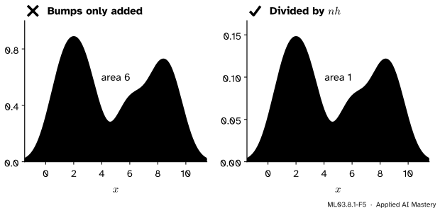
Wrong beside right. Adding the kernels without the factor \({1/(nh)}\) gives the right shape at the wrong scale: area 6, not 1.
“A kernel estimate is just the bumps added up.”
The bumps must also be scaled. Summing \({\kappa\big((x - x_i)/h\big)}\) alone gives area \({nh}\), here 6. The shape looks right, so the mistake hides until the curve is compared with another density or fed to a likelihood, where every log density is off by \({\ln(nh)}\).
“A density above 1 is a bug, since probabilities cannot exceed 1.”
A density is not a probability; an area under it is. With \({h = 0.05}\) the estimate of the six values rises to 1.33 over each point, and its total area is still 1. Read \(\hat f(x)\) as probability per unit of \(x\).
“Data that cannot be negative get an estimate that is zero below 0.”
Not with a Gaussian kernel. Its bumps spill over any boundary: for the six values with \({h = 1}\), \({3.0\%}\) of the estimate’s area lies below 0, from the bumps on 1 and 2. For waiting times, prices or counts, a kernel estimate puts mass where no value can be. Near a boundary the estimate is also biased low, and fixes such as reflecting the data or taking logs first exist for this reason.
Check yourself
Recall
1. Name the two faults of a histogram as a density estimate.
Show answer
It depends on the bin origin, which the data do not determine, and it is a staircase: flat inside bins and jumping at their edges.
2. Write the kernel density estimate with kernel \(\kappa\) and bandwidth \(h\).
3. Which substitution shows that each term of the estimate has area \({1/n}\)?
Show answer
\({u = (x - x_i)/h}\), so \({dx = h\,du}\); the factor \(h\) cancels the \({1/h}\) and leaves \({\tfrac1n \int \kappa(u)\,du = \tfrac1n}\).
4. What does KernelDensity.score_samples return?
Show answer
The logarithm of the estimated density at each point, so np.exp of it gives the density.
5. How do you make scipy.stats.gaussian_kde use the bandwidth \({h = 1}\) on one-dimensional data?
Show answer
Pass bw_method = 1 / s, where \(s\) is the sample standard deviation with \({n - 1}\) in the denominator, because SciPy’s kernel standard deviation is the factor times \(s\).
Exercises
1.★ Compute \({\hat f_1(6)}\) for the six values with the Gaussian kernel.
Show solution
The distances from 6 are 5, 4, 3, 0, 2 and 3. The kernel values are \({\varphi(5) = 0.0000}\), \({\varphi(4) = 0.0001}\), \({\varphi(3) = 0.0044}\), \({\varphi(0) = 0.3989}\), \({\varphi(2) = 0.0540}\) and \({\varphi(3) = 0.0044}\). Their sum, taken before rounding, is 0.4619, so \({\hat f_1(6) = 0.4619 / 6 = 0.0770}\). The point 6 stands alone, so its own bump supplies almost all of the height.
2.★★ With \({h = 2}\), compute the Epanechnikov and the tophat estimates of the six values at \({x = 2}\).
Show solution
The scaled distances \({(2 - x_i)/2}\) are 0.5, 0, \({-0.5}\), \({-2}\), \({-3}\) and \({-3.5}\); only the first three lie in \({[-1, 1]}\). Epanechnikov: \({0.75(1 - 0.25) = 0.5625}\), then 0.75, then 0.5625, which sum to 1.875, so
Tophat: three points each give one half, a sum of 1.5, so \({\hat f_2(2) = 1.5/12 = 0.125}\).
3.★★★ Show that a kernel estimate has mean \({\bar x}\), the sample mean, and variance \({\tfrac1n \sum_i (x_i - \bar x)^2 + h^2 \sigma_\kappa^2}\), where \({\sigma_\kappa^2 = \int u^2 \kappa(u)\,du}\). Evaluate both for the six values with the Gaussian kernel and \({h = 1}\).
Show solution
Use the substitution \({x = x_i + hu}\) in each term. For the mean,
So smoothing adds \({h^2 \sigma_\kappa^2}\) to the spread. For the six values \({\bar x = 29/6 = 4.833}\), the squared deviations sum to 54.833, so the variance is \({54.833/6} + 1 = 9.139 + 1 = 10.139\) (the Gaussian kernel has \({\sigma_\kappa^2 = 1}\)).
Summary card
A kernel estimate is a bump of area \(1/n\) on every point, added up.
ML03.8.1-F1
Bumps on points, summed.
Estimate:\({\hat f_h(x)} = {\frac{1}{nh}\sum_i \kappa\big((x - x_i)/h\big)}\), with \({\kappa \ge 0}\) and \({\int\kappa = 1}\).
Kernels: Gaussian, Epanechnikov \({\tfrac34(1 - u^2)}\) and tophat \({\tfrac12}\) on \({[-1, 1]}\).
Area 1: substitute \({u = (x - x_i)/h}\); the \(h\) from \({dx}\) cancels the \({1/h}\).
Better than a histogram: no bin origin, and smooth when the kernel is smooth.
In code:KernelDensity(bandwidth=h).score_samples gives the log density.
Sources and next steps
Sources. Each was opened and checked against this lesson on 15 November 2026.
T. Hastie, R. Tibshirani and J. Friedman, The Elements of Statistical Learning, 2nd edition, corrected 12th printing. Section 6.6.1: the local count in a neighbourhood of width \(\lambda\) (equation 6.21), described as bumpy, and the smooth Parzen estimate (6.22); with the Gaussian kernel the estimate is the empirical distribution convolved with a normal density (6.23), “adding independent Gaussian noise to each observation”.
L. Wasserman, Density Estimation, lecture notes for 36-708, Carnegie Mellon University. Section 3 on histograms and Section 4 on the kernel estimator, with the Epanechnikov kernel \({\tfrac34(1 - x^2)}\) on \({[-1, 1]}\); Section 4.5 on the bias near a boundary and its fixes (reflection, transformations, boundary kernels).
scikit-learn, Density Estimation, User Guide Section 2.8.2, with the Gaussian, tophat and Epanechnikov kernels, and the KernelDensity reference: score_samples returns the “log-likelihood of each sample”, normalised as a density.
SciPy, scipy.stats.gaussian_kde: a scalar bw_method is the bandwidth factor, and the kernel covariance is the data covariance (np.cov) times the factor squared.
Next.ML03.8.2 Choosing the bandwidth asks which \(h\) to use, derives the bias and variance that pull it in opposite directions, and lets the data choose it.