\( \newcommand{\vect}[1]{\boldsymbol{\mathbf{#1}}} \newcommand{\mat}[1]{\boldsymbol{\mathbf{#1}}} \newcommand{\R}{\mathbb{R}} \newcommand{\E}{\mathbb{E}} \newcommand{\Prob}{\mathbb{P}} \newcommand{\T}{^{\top}} \newcommand{\norm}[1]{\lVert #1 \rVert} \newcommand{\abs}[1]{\lvert #1 \rvert} \newcommand{\ihat}{\mkern1mu\hat{\boldsymbol{\imath}}\mkern2mu} \newcommand{\jhat}{\mkern1mu\hat{\boldsymbol{\jmath}}\mkern2mu} \newcommand{\pd}[2]{\frac{\partial #1}{\partial #2}} \newcommand{\argmax}{\operatorname*{arg\,max}} \newcommand{\argmin}{\operatorname*{arg\,min}} \newcommand{\cdata}[1]{\class{c-data}{#1}} \newcommand{\cmodel}[1]{\class{c-model}{#1}} \newcommand{\ctruth}[1]{\class{c-truth}{#1}} \newcommand{\cgrad}[1]{\class{c-grad}{#1}} \newcommand{\closs}[1]{\class{c-loss}{#1}} \newcommand{\cparam}[1]{\class{c-param}{#1}} \newcommand{\csecond}[1]{\class{c-second}{#1}} \renewcommand{\,}{\mkern3mu} \)

The EM algorithm, step by step

Fit a Gaussian mixture by alternating two easy steps: share each point between the components, then refit each component to its share. Derive both steps, run one full iteration by hand on the six values, and code it safely with log-sum-exp.

ML03.4.2L2 Intermediate25 min

In review

The maths and code on this page are checked by automated tests on every change, but an independent reader has not signed it off yet. Spot a mistake or a confusing step? Tell us.

Before this lesson: ML03.4.1 A mixture of Gaussians

What you will be able to do

Carry out the E-step: compute every responsibility with the parameters held fixed.
Derive the M-step updates for the weights, means and variances by differentiating the responsibility-weighted log-likelihood.
Run one full EM iteration by hand on the six values and check that the log-likelihood rises.
Implement EM in one dimension with log-sum-exp, and match it against scikit-learn’s GaussianMixture.

The question

The last lesson ended in a circle. The best mean for a component is a weighted average of the points, but the weights are the responsibilities, and those depend on the mean. You cannot solve for one without the other. What happens if you simply freeze the weights, solve, recompute the weights, and go round again?

From the last lesson

1. What is the responsibility \(r_{ik}\), and what do the responsibilities of one point add up to?

Show answer

The posterior probability that point \(i\) came from component \(k\), \({r_{ik} = \pi_k N(x_i \mid \mu_k, \sigma_k^2) / p(x_i)}\). Over the components they add to 1.

2. Under the start \({\pi = (\tfrac12, \tfrac12)}\), \({\mu = (2, 8)}\), \({\sigma^2 = (4, 4)}\), how is the value 6 shared?

Show answer

\({r_{41} = 0.1824}\) and \({r_{42} = 0.8176}\): about 18% component 1 and 82% component 2.

Intuition

Break the circle into two half-steps, each of which is easy on its own.

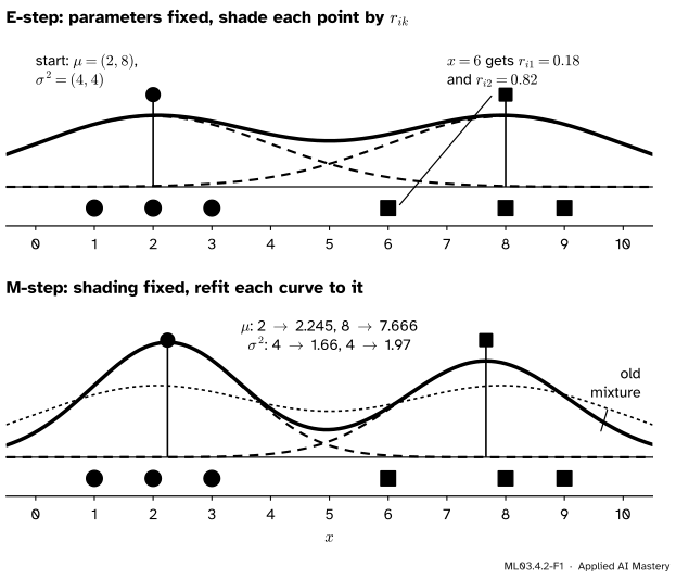
E-step. Hold the parameters fixed and shade every point by its responsibilities. This is Bayes’ rule, exactly as in the last lesson.
M-step. Hold the shading fixed and refit each component to the points, counting each point by its share. A point that is 18% component 1 counts as 0.18 of a point for component 1.

ML03.4.2-F1

One iteration of EM on the six values. The E-step shades each point by how much each component explains it. The M-step refits each curve to its shaded points: both narrow, and the left one moves right because 6 pulls on it with weight 0.18.

Then repeat. Each half-step is a short calculation; the circle is broken because each one uses only what the other produced. The name EM comes from the two steps: expectation and maximisation. It is the algorithm behind GaussianMixture, behind hidden Markov models and behind the topic models of ML03.7.

Build it up

Step 1. If the labels were known, fitting would be easy. Suppose we knew that 1, 2, 3 came from component 1 and 6, 8, 9 from component 2. Maximum likelihood (S02.3) would fit each component to its own points alone: the mean of each group, the variance of each group, and the weight as the share of points. Component 1 would get mean 2 and variance \(\tfrac23\); component 2 mean 7.667 and variance 1.556; each weight \(\tfrac12\).

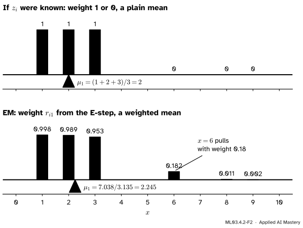
Step 2. Write the known labels as weights of 0 or 1. Give point \(i\) the weight 1 for its own component and 0 for the other. Then a group’s mean is \({\sum_i w_{ik} x_i / \sum_i w_{ik}}\), a weighted average over all the points.

Step 3. Replace the 0s and 1s by responsibilities. We do not know the labels, but the E-step gives the next best thing, the probability of each label. Use \(r_{ik}\) as the weight. Every point now pulls on every mean, in proportion to its share.

ML03.4.2-F2

The mean of component 1 as a balance point. With hard labels only 1, 2 and 3 carry weight and the balance sits at 2. With responsibilities, 6 adds a weight of 0.18 far to the right and the balance moves to 2.245.

Step 4. Recompute, and repeat. The new parameters give new responsibilities, which give new parameters. The next lesson proves that this never makes the fit worse.

The formal statement

The EM algorithm for a Gaussian mixture in one dimension

Start from any weights, means and variances. Then repeat until the log-likelihood \(\ell\) stops changing:

E-step. For every point and component,

\[ r_{ik} = \frac{\cparam{\pi_k}\, N(x_i \mid \cparam{\mu_k}, \cparam{\sigma_k^2})} {\sum_{j} \cparam{\pi_j}\, N(x_i \mid \cparam{\mu_j}, \cparam{\sigma_j^2})} . \]

M-step. With \({N_k = \sum_i r_{ik}}\), the effective number of points of component \(k\),

\[ \begin{aligned} \cparam{\pi_k} &= \frac{N_k}{n}, \qquad \cparam{\mu_k} = \frac{1}{N_k} \sum_{i} r_{ik}\, x_i, \\ \cparam{\sigma_k^2} &= \frac{1}{N_k} \sum_{i} r_{ik}\, (x_i - \cparam{\mu_k})^2 , \end{aligned} \]

where the variance uses the new mean.

What the M-step maximises. If the labels were known, the log-likelihood of the points and their labels (the complete-data log-likelihood) would be a sum of one term per point, the term of its own component. With the 0-or-1 label indicator \({[z_i = k]}\),

\[ \begin{aligned} &\sum_{i} \sum_{k} [z_i = k] \\ &\quad \times \big( \ln \pi_k + \ln N(x_i \mid \mu_k, \sigma_k^2) \big). \end{aligned} \]

EM replaces each indicator by its expected value given the data, which is \(r_{ik}\). So the M-step maximises

\[ \begin{aligned} Q &= \sum_{i} \sum_{k} r_{ik} \\ &\quad \times \big( \ln \pi_k + \ln N(x_i \mid \mu_k, \sigma_k^2) \big), \end{aligned} \]

with the \(r_{ik}\) held fixed. There is no sum inside a logarithm any more, so each parameter can be solved for directly. Lesson ML03.4.3 proves that raising \(Q\) raises \(\ell\).

The mean. The log of a normal density is

\[ \begin{aligned} \ln N(x \mid \mu, \sigma^2) &= -\tfrac12 \ln(2\pi\sigma^2) \\ &\quad - \frac{(x - \mu)^2}{2\sigma^2}. \end{aligned} \]

Only the terms with index \(k\) depend on \(\mu_k\). Their derivative is

\[ \pd{Q}{\mu_k} = \sum_i r_{ik}\, \frac{x_i - \mu_k}{\sigma_k^2}. \]

Setting it to zero and multiplying by \(\sigma_k^2\) gives \({\sum_i r_{ik} x_i = \mu_k N_k}\): the weighted mean. This time the \(r_{ik}\) are fixed numbers, so it is an answer.

The variance. Treat \({s = \sigma_k^2}\) as the unknown. The terms of \(Q\) that contain it are

\[ \sum_i r_{ik} \Big( -\tfrac12 \ln s - \frac{(x_i - \mu_k)^2}{2s} \Big). \]

Differentiate with respect to \(s\):

\[ \begin{aligned} \pd{Q}{s} &= \sum_i r_{ik} \Big( -\frac{1}{2s} \\ &\qquad + \frac{(x_i - \mu_k)^2}{2s^2} \Big). \end{aligned} \]

Multiply by \({2s^2}\) and set to zero: \({-s N_k + \sum_i r_{ik}(x_i - \mu_k)^2 = 0}\), the weighted variance. Because the mean that maximises \(Q\) is the same whatever \(s\) is, the variance uses that new mean.

The weights. The terms of \(Q\) with weights are \({\sum_k N_k \ln \pi_k}\), and the weights must add to 1. With two components, put \({\pi_2 = 1 - \pi_1}\) and maximise \({N_1 \ln \pi_1 + N_2 \ln(1 - \pi_1)}\). Its derivative is

\[ \begin{aligned} &\frac{N_1}{\pi_1} - \frac{N_2}{1 - \pi_1} = 0 \\ &\quad\Longrightarrow\quad \pi_1 = \frac{N_1}{N_1 + N_2} = \frac{N_1}{n}, \end{aligned} \]

where \({N_1 + N_2 = n}\) because the responsibilities of each point add to 1. With \(K\) components the same answer, \({\pi_k = N_k / n}\), comes from a Lagrange multiplier (M08.7).

A fixed point of EM solves the last lesson’s equation. When EM stops moving, the means it returns satisfy \({\mu_k = \sum_i r_{ik} x_i / N_k}\) with responsibilities computed from those same means: exactly the stationary condition \({\pd{\ell}{\mu_k} = 0}\) that had no closed form. EM solves it by going round the circle until it closes.

ML03.4.2-F4

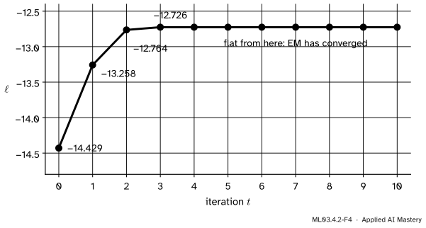
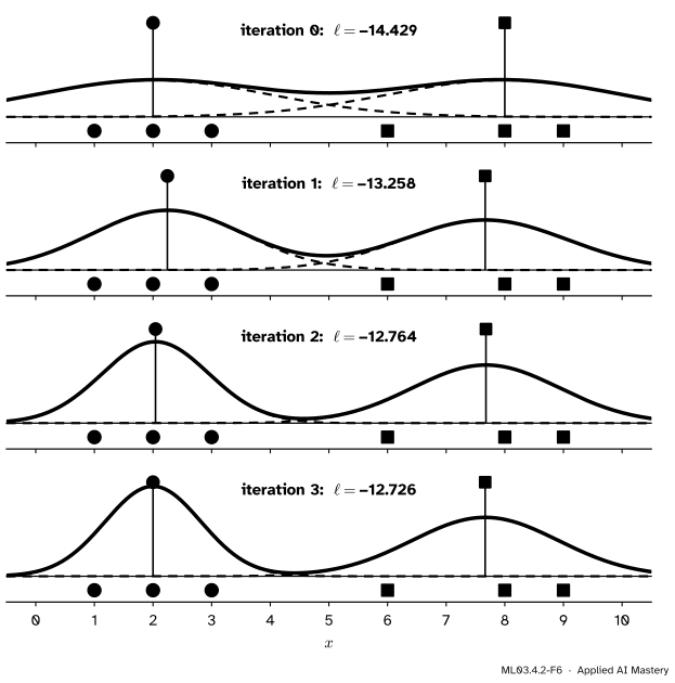
The log-likelihood of the six values after each EM iteration. It rises fast, then levels off at about \(-12.726\), with means near 2 and 7.665 and variances near \(\tfrac23\) and 1.565.

Worked example

Run one full EM iteration on the six values from the start \({\pi = (\tfrac12, \tfrac12)}\), \({\mu = (2, 8)}\), \({\sigma^2 = (4, 4)}\).

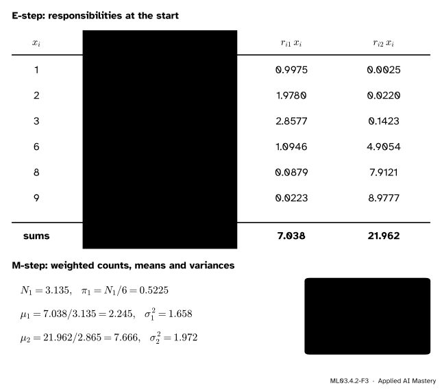
E-step. The responsibilities of component 1 are \({\sigma(7.5 - 1.5x_i)}\) (last lesson): 0.9975, 0.9890, 0.9526, 0.1824, 0.0110 and 0.0025. Those of component 2 are one minus these.

Effective counts and weights. Add each column: \({N_1 = 3.135}\) and \({N_2 = 2.865}\), which add to 6. So \({\pi_1 = 3.135/6 = 0.5225}\) and \({\pi_2 = 0.4775}\).

Means. Multiply each \(r_{i1}\) by \(x_i\) and add:

\[ \begin{aligned} &\textstyle\sum_i r_{i1} x_i \\ &\quad = 0.9975 + 1.9780 + 2.8577 \\ &\quad\quad + 1.0946 + 0.0879 + 0.0223 \\ &\quad = 7.038, \end{aligned} \]

so \({\mu_1 = 7.038 / 3.135 = 2.245}\). The same for component 2 gives \({\mu_2 = 21.962 / 2.865 = 7.666}\).

Variances. It is quicker to use \({\sigma_k^2 = \sum_i r_{ik} x_i^2 / N_k - \mu_k^2}\), the weighted form of “mean of the squares minus the square of the mean”. For component 1, \({\sum_i r_{i1} x_i^2 = 20.998}\), so

\[ \begin{aligned} \sigma_1^2 &= 20.998 / 3.135 - 2.245^2 \\ &= 6.698 - 5.040 = 1.658 . \end{aligned} \]

For component 2, \({\sum_i r_{i2} x_i^2 = 174.002}\), so \({\sigma_2^2 = 60.733 - 58.762 = 1.972}\).

ML03.4.2-F3

The worked-example trace. The column sums give the effective counts and the weighted sums; the M-step divides one by the other. The log-likelihood rises from \(-14.429\) to \(-13.258\).

Check. Under the new parameters the log-likelihood is \(-13.258\), up from \(-14.429\). One more iteration gives \(-12.764\), and a third \(-12.726\), after which it barely moves.

Code

From scratch, working with logarithms throughout. The E-step adds probabilities stored as logs with logsumexp, which subtracts the largest log before exponentiating, so nothing underflows.

import numpy as np
from scipy.special import logsumexp

x = np.array([1.0, 2.0, 3.0, 6.0, 8.0, 9.0])

def log_normal(x, mu, var):
    return -0.5 * (np.log(2 * np.pi * var) + (x - mu) ** 2 / var)

def e_step(x, pi, mu, var):
    log_t = np.log(pi) + log_normal(x[:, None], mu, var)      # n by K
    log_p = logsumexp(log_t, axis=1)                           # log p(x_i)
    return np.exp(log_t - log_p[:, None]), log_p.sum()         # r and the log-likelihood

def m_step(x, r):
    n_k = r.sum(axis=0)
    mu = (r * x[:, None]).sum(axis=0) / n_k
    var = (r * (x[:, None] - mu) ** 2).sum(axis=0) / n_k       # uses the new mean
    return n_k / len(x), mu, var

pi, mu, var = np.array([0.5, 0.5]), np.array([2.0, 8.0]), np.array([4.0, 4.0])
trace = []
for it in range(50):
    r, ell = e_step(x, pi, mu, var)        # ell is the log-likelihood of the current parameters
    trace.append(ell)
    if it == 0:
        r_first = r
    pi, mu, var = m_step(x, r)
    if it == 0:
        print("after one iteration:", pi.round(4), mu.round(3), var.round(3))
print("log-likelihood:", np.round(trace[:4], 3))
print("settles at:", pi.round(3), mu.round(3), var.round(3))

after one iteration: [0.5225 0.4775] [2.245 7.666] [1.658 1.972]
log-likelihood: [-14.429 -13.258 -12.764 -12.726]
settles at: [0.5 0.5] [2.    7.665] [0.667 1.565]

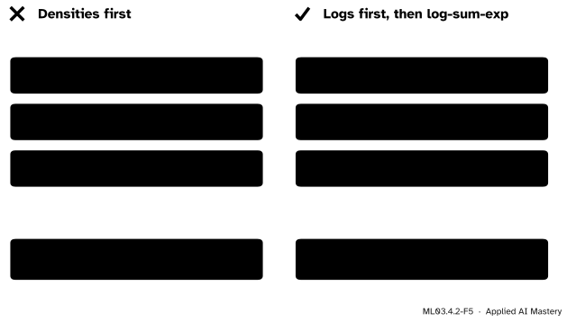
Why logs matter: put one point at 50 and give the components variance 1. Both densities are far below the smallest positive float, and the naive E-step divides zero by zero.

far = np.array([50.0])
with np.errstate(invalid="ignore"):
    dens = 0.5 * np.exp(-(far[:, None] - [2.0, 8.0]) ** 2 / 2) / np.sqrt(2 * np.pi)
    naive = dens / dens.sum(axis=1, keepdims=True)
safe, _ = e_step(far, np.array([0.5, 0.5]), np.array([2.0, 8.0]), np.array([1.0, 1.0]))
print("densities:", dens, " naive r:", naive, " log-sum-exp r:", safe)

densities: [[0. 0.]]  naive r: [[nan nan]]  log-sum-exp r: [[5.50161108e-118 1.00000000e+000]]

Now the library. GaussianMixture runs the same E and M steps. Give it our start through weights_init, means_init and precisions_init (precision is one over the variance), turn off its tiny variance floor with reg_covar=0, and stop it after a set number of iterations.

import warnings
from sklearn.mixture import GaussianMixture
from sklearn.exceptions import ConvergenceWarning

for steps in (1, 2, 3):
    gm = GaussianMixture(n_components=2, covariance_type="spherical", weights_init=[0.5, 0.5],
                         means_init=[[2.0], [8.0]], precisions_init=[0.25, 0.25],
                         reg_covar=0.0, tol=0.0, max_iter=steps)
    with warnings.catch_warnings():
        warnings.simplefilter("ignore", ConvergenceWarning)
        gm.fit(x[:, None])
    print(steps, gm.means_.ravel().round(3), gm.covariances_.round(3),
          round(gm.score(x[:, None]) * len(x), 3))

1 [2.245 7.666] [1.658 1.972] -13.258
2 [2.043 7.679] [0.833 1.572] -12.764
3 [2.    7.665] [0.668 1.564] -12.726

score returns the average log-likelihood per point, so multiply by \(n\) to compare with \(\ell\). With one feature, "spherical" means one variance per component.

Explore

ML03.4-X1

EM stepper

Press E-step to shade the points and M-step to refit the curves, or Step for both and Play to run. Switch to In the plane for clusters drawn as ellipses, change \(K\), and try Random start a few times.

Three things to try. On the six values, press E-step and then M-step and check the read-out against the worked example. Set \(K = 3\) on the six values and play: one component shrinks onto the single value 6 until the stepper’s variance floor of 0.01 stops it, and \(\ell\) ends near \(-9.78\). That is a higher number but not a better model, and lesson ML03.4.3 explains why. Then, in the plane with the tilted blobs and \(K = 3\), press Random start several times and note the final \(\ell\): different starts can stop at different answers, which lesson ML03.4.3 explains.

Pitfalls

ML03.4.2-F5

Wrong beside right, for a point at 50 and components of variance 1. Both densities underflow to 0.0 and the naive responsibility is \(0/0\). In logs the larger term is factored out first, and the answer is clean.

“I can compute the densities and divide; the logs are only for speed.”

Densities far in a component’s tail fall below about \(5 \times 10^{-324}\), the smallest positive double, and become exactly 0. With several features this happens to ordinary points, because the log densities add up across features. Work with \({\ln \pi_k + \ln N}\) and combine with log-sum-exp, as the code does.

“In the M-step the variance should use the old mean, since the responsibilities came from the old parameters.”

The variance that maximises \(Q\) uses the new mean. Around any other centre \(a\) the weighted spread is larger by the square of the distance between the centres (exercise 2):

\[ \begin{aligned} &\frac{1}{N_k}\sum_i r_{ik}(x_i - a)^2 \\ &\quad = \sigma_k^2 + (\mu_k - a)^2 . \end{aligned} \]

From the start, component 1 would get 1.718 instead of 1.658.

“Each weight is \(N_k\) over the number of components.”

The weight is \({N_k / n}\), the effective share of the points. Dividing the variance by \(n\) instead of \(N_k\) is the twin mistake: it shrinks every variance by the component’s weight.

Check yourself

Recall

1. What is held fixed in the E-step, and what is computed?

Show answer

The weights, means and variances are held fixed; the responsibilities \(r_{ik}\) are computed by Bayes’ rule.

2. Write the M-step updates for \(\pi_k\), \(\mu_k\) and \(\sigma_k^2\).

Show answer

With \({N_k = \sum_i r_{ik}}\): \({\pi_k = N_k / n}\), \({\mu_k = \sum_i r_{ik} x_i / N_k}\) and \({\sigma_k^2 = \sum_i r_{ik}(x_i - \mu_k)^2 / N_k}\), using the new \(\mu_k\).

3. What does the M-step maximise, and why is that easy?

Show answer

\(Q\), the complete-data log-likelihood with each label indicator replaced by its expected value \(r_{ik}\), with the \(r_{ik}\) held fixed. No sum sits inside a logarithm, so each parameter is found by setting one derivative to zero.

4. After one iteration from the start, what are the new means, and what is the log-likelihood?

Show answer

\({\mu = (2.245, 7.666)}\) and \({\ell = -13.258}\), up from \(-14.429\).

5. Why does the code use logsumexp in the E-step?

Show answer

Densities in the tails underflow to 0, giving \({0/0}\). Working with log densities and log-sum-exp, which factors out the largest term first, keeps every responsibility finite and accurate.

Exercises

1. ★ From the table of the worked example, check that \({N_1 + N_2 = 6}\) and that \({\pi_1\mu_1 + \pi_2\mu_2}\) equals the plain mean of the six values. Why must both hold after every M-step?

Show solution

\({3.135 + 2.865 = 6}\). And

\[ \begin{aligned} &0.5225 \times 2.245 + 0.4775 \times 7.666 \\ &\quad = 1.173 + 3.661 = 4.833, \end{aligned} \]

the mean of 1, 2, 3, 6, 8, 9, which is \({29/6 = 4.833}\). The first holds because each point’s responsibilities add to 1. The second because \({\pi_k \mu_k = \tfrac{1}{n}\sum_i r_{ik} x_i}\), so

\[ \begin{aligned} \sum_k \pi_k \mu_k &= \frac1n \sum_i x_i \sum_k r_{ik} \\ &= \frac1n \sum_i x_i . \end{aligned} \]

2. ★★ Show that the weighted spread about any number \(a\) is \({\sigma_k^2 + (\mu_k - a)^2}\), that is, \({\tfrac{1}{N_k}\sum_i r_{ik}(x_i - a)^2}\) equals it for every \(a\), where \(\mu_k\) and \(\sigma_k^2\) are the M-step values. Use it to find the variance component 1 would get from the start if the old mean 2 were used.

Show solution

Write \({x_i - a = (x_i - \mu_k) + (\mu_k - a)}\) and square:

\[ \begin{aligned} (x_i - a)^2 &= (x_i - \mu_k)^2 \\ &\quad + (\mu_k - a)^2 \\ &\quad + 2(x_i - \mu_k)(\mu_k - a). \end{aligned} \]

Multiply by \(r_{ik}\), add over \(i\) and divide by \(N_k\). The first term gives \(\sigma_k^2\) and the second \({(\mu_k - a)^2}\). The last gives zero, because \(\mu_k\) is the weighted mean:

\[ \frac{2(\mu_k - a)}{N_k} \sum_i r_{ik}(x_i - \mu_k) = 0 . \]

With \({a = 2}\): \({1.658 + 0.245^2 = 1.718}\).

3. ★★★ Suppose every responsibility is exactly 0 or 1, each point going wholly to its nearest mean. Show that the M-step for the means is then the update step of k-means (ML03.1), and say which part of k-means the E-step has become.

Show solution

If \({r_{ik} \in \{0, 1\}}\), then \({N_k}\) is the number of points with \({r_{ik} = 1}\), and \({\mu_k = \sum_i r_{ik} x_i / N_k}\) is the plain mean of those points: the k-means update. The E-step has become the assignment step, sending each point wholly to its nearest centre. Lesson ML03.4.3 shows exactly when soft responsibilities turn into these hard ones: when all components share a variance that shrinks to zero.

Summary card

EM: shade the points, refit the curves, repeat.

The anchor figure again: the E-step panel with wide bells at 2 and 8 and the six values shaded, and the M-step panel with the bells refitted, narrower and moved to 2.245 and 7.666. — ML03.4.2-F1
E shades, M refits.

E-step. \({r_{ik} \propto \pi_k N(x_i \mid \mu_k, \sigma_k^2)}\), normalised over \(k\).
M-step. \({N_k = \sum_i r_{ik}}\), \({\pi_k = N_k / n}\), \({\mu_k = \sum_i r_{ik} x_i / N_k}\).
Variance. \({\sigma_k^2 = \sum_i r_{ik}(x_i - \mu_k)^2 / N_k}\), with the new mean.
Six values. \(\ell\): \(-14.429\), \(-13.258\), \(-12.764\), \(-12.726\).

Sources and next steps

Sources. Each was opened and checked against this lesson on 15 November 2026.

Christopher M. Bishop, Pattern Recognition and Machine Learning, Springer 2006. Section 9.2.2: the stationary condition for the means (9.16), the updates (9.17) to (9.19) with \(N_k\) as “the effective number of points assigned to cluster \(k\)”, the Lagrange multiplier for the weights (9.20) to (9.22), the remark that these “do not constitute a closed-form solution”, and the order of the M-step, new means first and then the covariances.
T. Hastie, R. Tibshirani and J. Friedman, The Elements of Statistical Learning, 2nd edition, corrected 12th printing (2017). Section 8.5.1: the complete-data log-likelihood (8.40), each label replaced by its expected value, the responsibility (8.41), and Algorithm 8.1 with its weighted means and variances.
scikit-learn, sklearn.mixture.GaussianMixture, version 1.9.1: weights_init, means_init, precisions_init (the inverse covariances), reg_covar (default \(10^{-6}\), added to the diagonal), tol, max_iter, and score as the per-sample average log-likelihood.

Next. ML03.4.3 Why EM climbs proves that the log-likelihood never falls, finds k-means inside EM, and shows how EM can still go wrong.

This lesson unlocks

ML03.4.3 Why EM climbs

Your progress is saved in this browser only. No account, no tracking.