With no labels to check against, a clustering has to be judged by a score. Meet the k-means objective J, the sum of squared distances from points to their centres, and derive its two facts: the best centre is the mean, and the best cluster for a point is its nearest centre.
ML03.1.1L2 Intermediate25 minIn review (what this means)
The maths and code on this page are checked by automated tests on every change, but an independent reader has not signed it off yet. Spot a mistake or a confusing step? Tell us.
Explain what clustering is used for and why, without labels, a grouping has to be judged by an objective.
Compute the k-means objective J by hand for a grouping and its centres.
Derive, by setting the gradient to zero, that the best centre for a fixed cluster is the mean of its points.
Show that for fixed centres each point should join its nearest centre, and describe the Voronoi cells and straight borders this creates.
The question
A shop has ten thousand customers and a record of what each one buys. Nobody has labelled them, yet the marketing team wants four groups of similar customers. There is no answer key to mark a grouping against. So what makes one grouping better than another?
Intuition
Clustering splits a set of examples into groups, called clusters, so that examples in the same cluster are alike. It has many uses: customer segments, the few colours that best stand for a photo, piles of documents on the same topic. In every case there are no labels. That is what makes it unsupervised learning: no target \(y\) says what the right answer was.
Without labels, we cannot count mistakes. Instead we write down a score for how tight a grouping is and look for the grouping with the best score. k-means uses the simplest score there is. Give each cluster a centre, measure how far each point is from its own centre, square those distances and add them up.
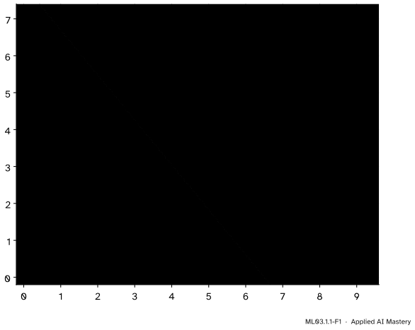
ML03.1.1-F1
The nine points of this course split into two clusters. Each orange cross is a centre, each reddish-purple line runs from a point to its own centre, and \(J\) adds up the squares of their lengths. The tints show which centre is nearer, everywhere in the plane.
A small \(J\) means every point sits close to its centre: the clusters are tight. The picture holds the two questions this lesson answers. Given the clusters, where should each centre go? Given the centres, which cluster should each point join?
Build it up
Step 1. A clustering is an assignment. We have \(n\) points \(\vect{x}_1, \dots, \vect{x}_n\) in \(\R^d\) and want \(K\) clusters, numbered \(k = 1, \dots, K\). A clustering says, for each point \(i\), which cluster it is in. Write that number as \(z_i\). For the nine points in the anchor figure, the four lower points have \(z_i = 1\) and the other five have \(z_i = 2\).
Step 2. Each cluster gets a centre. The centre \(\vect{\mu}_k\) is a point in \(\R^d\) that stands for the whole cluster. It need not be one of the data points. In the figure the centres are \((1.5, 1.5)\) and \((6, 5.2)\).
Step 3. Score the fit by squared distance. A point \(\vect{x}_i\) in cluster \(z_i\) is represented by the centre \(\vect{\mu}_{z_i}\), and the squared distance between them is the cost of that point. Add the costs over all points and you have \(J\).
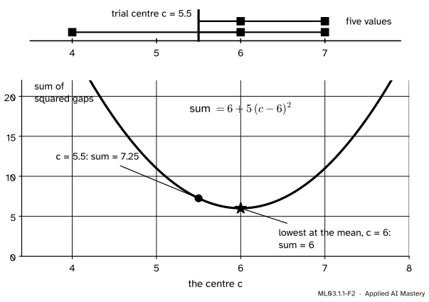
Step 4. Two questions, one at a time.\(J\) depends on two things: the assignments and the centres. Hold the assignments fixed and ask where the centres should go. Look at one cluster and one coordinate first: the five \(x\)-coordinates of cluster 2 are \(4, 6, 6, 7, 7\).
ML03.1.1-F2
For the values \(4, 6, 6, 7, 7\), the sum of squared gaps to a centre \(c\) is a bowl. Its lowest point is at the mean, \(c = 6\). Moving the centre to \(5.5\) raises the sum from \(6\) to \(7.25\).
The bowl has one lowest point, and it sits at the mean of the five values. The next section proves that this is no accident, in any number of dimensions.
The formal statement
NoteDefinition: the k-means objective
Given points \(\vect{x}_1, \dots, \vect{x}_n\) in \(\R^d\), assignments \(z_i \in \{1, \dots, K\}\) and centres \(\vect{\mu}_1, \dots, \vect{\mu}_K\), the k-means objective (also called the within-cluster sum of squares, the distortion, or in scikit-learn the inertia) is
Fact 1: for fixed assignments, the best centre is the mean. Only the points of cluster \(k\) involve \(\vect{\mu}_k\), so we can minimise one cluster at a time. Call its points \(C_k\) and their number \(n_k\). Write the squared distance as a dot product and expand:
Take the gradient with respect to \(\vect{\mu}\), one coordinate at a time as in M04.10. The first sum does not depend on \(\vect{\mu}\). The middle term is linear in \(\vect{\mu}\), and the gradient of \(\norm{\vect{\mu}}^2 = \mu_1^2 + \dots + \mu_d^2\) is \(2\vect{\mu}\). So
This is the mean of the cluster’s points, which is why the method is called k-means. It is a minimum and not a maximum: \(J_k\) is \(n_k \norm{\vect{\mu}}^2\) plus terms of lower degree, a bowl that opens upward in every direction, like the curve in the figure above.
Go deeper: the same fact without calculus, and a pairwise form of J
Write \(\bar{\vect{x}}\) for the mean of \(C_k\), and add and subtract it inside each term, so that \({\vect{x}_i - \vect{\mu}}\) becomes \({(\vect{x}_i - \bar{\vect{x}})} + {(\bar{\vect{x}} - \vect{\mu})}\). Expand the square:
The last term is never negative and is zero only at \(\vect{\mu} = \bar{\vect{x}}\). This identity is Lemma 2.1 of Arthur and Vassilvitskii. Applied to \(\norm{\vect{x}_j - \vect{x}_i}^2\) summed over all \(j\) in the cluster and then over all \(i\), it gives, for each cluster,
So minimising \(J\) is the same as making the average squared distance between points of the same cluster small.
Fact 2: for fixed centres, the best cluster is the nearest centre. Now hold the centres fixed. Each point appears in exactly one term of \(J\), and its term depends only on its own \(z_i\). So each point can be placed on its own, and its term is smallest when
Nearest-centre regions are Voronoi cells with straight borders. The set of all places that are nearer to \(\vect{\mu}_k\) than to any other centre is the Voronoi cell of \(\vect{\mu}_k\). The border between two centres is where the two squared distances are equal. Expand both sides:
What is left is linear in \(\vect{x}\). So the border is a straight line (a plane, in more dimensions) at right angles to the segment joining the centres, through its midpoint. Every cell is convex, with straight sides; a cell at the edge of the data runs off to infinity.
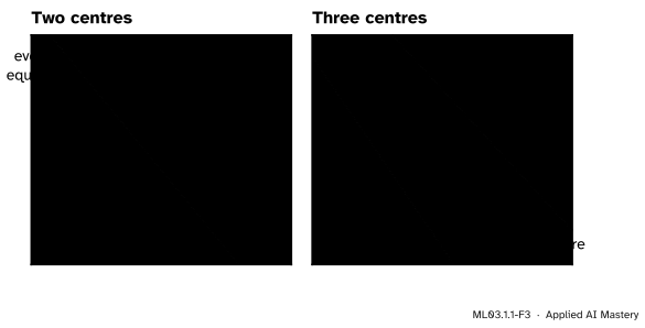
ML03.1.1-F3
Fixed centres split the plane into Voronoi cells. With two centres the border is the perpendicular bisector of the segment between them. The bridge point \((4, 4)\) is at squared distance \(12.5\) from one centre and \(5.44\) from the other, so it joins the second.
Worked example
Score the grouping of the anchor figure, then try the other place for the bridge point.
The centres. Cluster 1 is the lower square \((1, 1), (2, 1), (1, 2), (2, 2)\). Its mean is
The costs. Each point of the lower square is \(0.5\) away from \((1.5, 1.5)\) in each coordinate, so its squared distance is \({0.25 + 0.25} = 0.5\), and the four add to \(2\). For cluster 2, subtract \((6, 5.2)\) and square:
\((6, 5)\): \(0^2 + 0.2^2 = 0.04\)
\((7, 5)\): \(1^2 + 0.2^2 = 1.04\)
\((6, 6)\): \(0^2 + 0.8^2 = 0.64\)
\((7, 6)\): \(1^2 + 0.8^2 = 1.64\)
\((4, 4)\): \(2^2 + 1.2^2 = 5.44\)
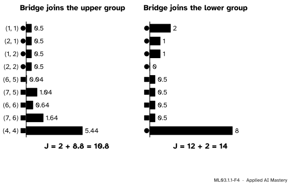
These add to \(8.8\), so \(J = 2 + 8.8 = 10.8\).
The other grouping. Move the bridge point to the lower group. The lower five now have mean \((10/5,\; 10/5) = (2, 2)\) and costs \(2, 1, 1, 0, 8\), which add to \(12\). The upper square alone has mean \((6.5, 5.5)\) and four costs of \(0.5\), which add to \(2\). So \(J = 12 + 2 = 14\).
ML03.1.1-F4
\(J\) by hand, one squared distance per point. With the bridge point in the upper group \(J = 10.8\); in the lower group \(J = 14\). The objective prefers the first grouping.
The objective has made a decision for us. The bridge point is nearer to the upper square in squared distance, so \(J\) is lower when it joins that group. Lesson ML03.1.2 shows that \(10.8\) is the lowest \(J\) of all 255 ways to split the nine points into two groups.
Code
First from scratch. A grouping is an array z of cluster numbers (from 0 in code), and the centres are the means of the groups.
import numpy as npX = np.array([(1, 1), (2, 1), (1, 2), (2, 2), (6, 5), (7, 5), (6, 6), (7, 6), (4, 4)], dtype=float)def centres_of(X, z, K):"""Fact 1: the best centre of each cluster is the mean of its points."""return np.array([X[z == k].mean(axis=0) for k inrange(K)])def J(X, z, C):"""The k-means objective: squared distance from each point to its own centre, summed."""return ((X - C[z]) **2).sum()up = np.array([0, 0, 0, 0, 1, 1, 1, 1, 1]) # the bridge point joins the upper groupdown = np.array([0, 0, 0, 0, 1, 1, 1, 1, 0]) # the bridge point joins the lower groupC_up, C_down = centres_of(X, up, 2), centres_of(X, down, 2)print("centres:", C_up.tolist(), " J =", round(J(X, up, C_up), 3))print("centres:", C_down.tolist(), " J =", round(J(X, down, C_down), 3))
Fact 1 can be checked numerically: nudge a centre in any direction and \(J\) goes up by \(n_k\) times the squared length of the nudge, exactly as the identity in the deeper block says.
rng = np.random.default_rng(0)for _ inrange(3): nudge = rng.normal(scale=0.3, size=2) C = C_up.copy() C[1] += nudgeprint(f"rise {J(X, up, C) - J(X, up, C_up):.4f} 5 x |nudge|^2 = {5* nudge @ nudge:.4f}")
rise 0.0150   5 x |nudge|^2 = 0.0150
rise 0.1895   5 x |nudge|^2 = 0.1895
rise 0.1880   5 x |nudge|^2 = 0.1880
Fact 2 is one line of NumPy: compute every squared distance from every point to every centre, then take the smallest in each row. scikit-learn offers the same as pairwise_distances_argmin.
from sklearn.metrics import pairwise_distances_argminD2 = ((X[:, None, :] - C_up[None, :, :]) **2).sum(axis=-1) # an n by K tablenearest = D2.argmin(axis=1)print("squared distances of (4, 4):", D2[8].round(2).tolist())print("nearest centre for each point:", nearest.tolist())print("scikit-learn agrees:", np.array_equal(nearest, pairwise_distances_argmin(X, C_up)))
squared distances of (4, 4): [12.5, 5.44]
nearest centre for each point: [0, 0, 0, 0, 1, 1, 1, 1, 1]
scikit-learn agrees: True
The grouping we chose by eye is also the one that the nearest-centre rule gives back: each point is already in the cell of its own centre. That self-consistency is what the next lesson’s algorithm looks for.
Explore
The module’s interactive, the k-means stepper, lives in the next lesson. To use it with this lesson, choose the nine points, set \(K = 2\), place two centres by clicking and press assign: the tinted cells are the Voronoi cells of your centres, and the read-out prints \(J\). Then press update and watch each centre jump to the mean of its points and \(J\) drop.
Pitfalls
ML03.1.1-F5
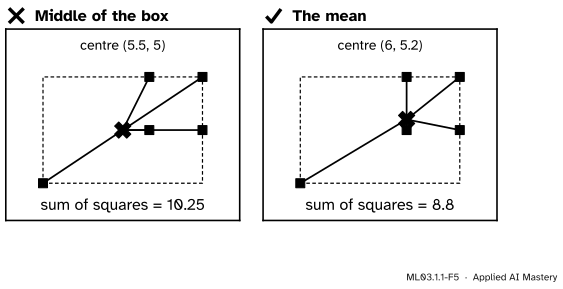
Wrong beside right. The middle of the cluster’s bounding box, \((5.5, 5)\), costs \(10.25\). The mean, \((6, 5.2)\), costs \(8.8\), the least possible.
“The centre of a cluster is the middle of its spread.”
The middle of the bounding box listens only to the two most extreme points. The mean listens to every point, and it is the one that minimises the sum of squares. The gap is exactly \(n_k \norm{\bar{\vect{x}} - \vect{\mu}}^2\): here \(5 \times (0.5^2 + 0.2^2) = 1.45\), the difference between \(10.25\) and \(8.8\).
“k-means makes the distances to the centres small.”
It makes the squared distances small. The point that minimises the sum of plain distances is a different point, the geometric median, which has no formula. Squaring is what makes the best centre the mean, and it is also why one far point costs so much: the bridge point alone, at \(5.44\), is about half of \(J = 10.8\). Lesson ML03.1.4 returns to what that does to outliers.
“A lower J means a better clustering, full stop.”
Only for the same data, the same features and the same \(K\). With one cluster per point \(J = 0\), and rescaling one feature changes every distance. Use \(J\) to compare groupings of one data set into the same number of clusters. Choosing \(K\) needs other tools, met in ML03.1.3.
Check yourself
Recall
1. Why is clustering called unsupervised learning?
Show answer
Because there are no labels: no target says which group each example truly belongs to, so the result cannot be marked against an answer key.
2. Write the k-means objective \(J\) in words.
Show answer
The sum, over all points, of the squared Euclidean distance from each point to the centre of the cluster it is assigned to.
3. With the assignments fixed, where should each centre go, and why?
Show answer
At the mean of its points. Setting the gradient of that cluster’s sum of squares to zero gives \(\vect{\mu}_k = \frac{1}{n_k}\sum_{i \in C_k} \vect{x}_i\).
4. With the centres fixed, which cluster should each point join?
Show answer
The cluster of its nearest centre, because each point’s term in \(J\) depends only on its own assignment.
5. What shape is the border between the Voronoi cells of two centres?
Show answer
A straight line (a plane in more dimensions): the perpendicular bisector of the segment that joins the two centres.
Exercises
1.★ One cluster holds the values \(2, 4, 9\) on a line. Find its best centre and its \(J\). Then find \(J\) if the centre is put at \(4\) instead.
Show solution
The best centre is the mean, \({(2 + 4 + 9)/3} = 5\). Then \(J = 3^2 + 1^2 + 4^2 = 9 + 1 + 16 = 26\). With the centre at \(4\), \(J = 2^2 + 0^2 + 5^2 = 29\). As a check, the identity of the deeper block predicts \(26 + 3 \times (5 - 4)^2 = 29\).
2.★★ Two centres sit at \((0, 0)\) and \((4, 2)\). Find the equation of the border between their Voronoi cells, and decide which centre the point \((3, 0)\) joins.
so \(8x + 4y = 20\), which is \(2x + y = 5\). At \((3, 0)\), \(2x + y = 6 > 5\), which is the side of \((4, 2)\). Check with distances: the squared distance to \((0, 0)\) is \(9\) and to \((4, 2)\) it is \({1 + 4} = 5\). The point joins \((4, 2)\).
3.★★★ Prove that for any point \(\vect{c}\) and any cluster of \(n\) points with mean \(\bar{\vect{x}}\),
Sum over \(i\). The middle terms add to \(2\,(\bar{\vect{x}} - \vect{c})\) dotted with the sum of the deviations, and that sum is zero by the definition of the mean:
\[
\sum_i (\vect{x}_i - \bar{\vect{x}}) = \sum_i \vect{x}_i - n \bar{\vect{x}} = \vect{0}.
\] The last terms add to \(n \norm{\bar{\vect{x}} - \vect{c}}^2\), which proves the identity.
For cluster 2, \(\bar{\vect{x}} = (6, 5.2)\), the sum about the mean is \(8.8\) and \(n = 5\). With \(\vect{c} = (5.5, 5)\), \(\norm{\bar{\vect{x}} - \vect{c}}^2 = 0.25 + 0.04 = 0.29\), so the sum is \(8.8 + 5 \times 0.29 = 10.25\), as in the pitfall figure.
Summary card
k-means scores a grouping by the squared distances from points to their centres.
Sources. Each was opened and checked against this lesson on 15 November 2026.
Trevor Hastie, Robert Tibshirani and Jerome Friedman, The Elements of Statistical Learning, 2nd edition (free PDF from the authors). Section 14.3.6, K-means: the within-cluster scatter in its pairwise and centred forms (equation 14.31), the mean as the minimiser of a sum of squares (14.32), the nearest-mean assignment (14.34), and the name Voronoi tessellation for the nearest-centre regions.
Andrew Ng, CS229 lecture notes: The k-means clustering algorithm, Stanford University. Defines the distortion function \(J\) as the sum of squared distances from each example to its assigned centroid, and describes the two steps as minimising \(J\) in turn over the assignments and over the centroids.
David Arthur and Sergei Vassilvitskii, k-means++: The Advantages of Careful Seeding. Section 2 defines the potential \(\phi\), the k-means objective, and Lemma 2.1 is the identity of the deeper block and Exercise 3.
scikit-learn developers, User Guide, Section 2.3.2 K-means, version 1.9. Calls the objective the inertia, or within-cluster sum-of-squares criterion, and notes that it is not a normalised score: lower is better and zero is optimal.
Next.ML03.1.2 Lloyd’s algorithm alternates the two facts of this lesson and proves that \(J\) can only go down.