The output activation is fixed by the target; the hidden one is a choice. Race sigmoid, tanh, ReLU and GELU in the same network on make_moons, and derive why the backward signal through a stack of sigmoid layers shrinks by at least a factor of 4 per layer.
DL01.3.4L2 Intermediate25 minIn review (what this means)
The maths and code on this page are checked by automated tests on every change, but an independent reader has not signed it off yet. Spot a mistake or a confusing step? Tell us.
Choose the output activation from the kind of target: identity for a number, sigmoid for yes or no, softmax for one of K classes.
Derive that each sigmoid layer shrinks the backward signal by at least a factor of 4, up to the size of its weights.
Train the same network with different hidden activations in NumPy and compare their loss curves and decision boundaries.
Use the activation argument of scikit-learn’s MLPClassifier and read its results.
The question
You are about to train a small network on the two moons. There are at least seven activations to put in its hidden layers and three to put on its output. Which choices are decisions and which are forced, and how big a difference does the hidden choice really make when everything else is held fixed?
From the last lesson
1. Write SiLU and GELU as \(z\) times a gate.
Show answer
\({\operatorname{silu}(z) = z\,\sigma(z)}\) and \({\operatorname{gelu}(z) = z\,\Phi(z)}\), with \(\Phi\) the standard normal cumulative distribution function.
2. What is the derivative of softplus?
Show answer
The sigmoid, \({\sigma(z)}\).
Intuition
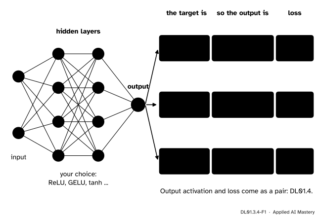
A network has two kinds of activation, and they are chosen for different reasons. The hidden activations shape how the network bends space and how well gradients flow back through it: a design choice. The output activation turns the last pre-activations into the kind of answer the target needs: not a choice at all, once the target is known.
DL01.3.4-F1
Hidden activations are a choice; the output activation is read off the target, and it comes with its loss.
For the output, ask what the target is. A real number that can be negative needs an output that can be any real number: the identity. A yes-or-no label needs a probability: the sigmoid. One of \(K\) classes needs \(K\) probabilities that add to 1: the softmax of ML01.6.4. Each comes paired with a loss, and DL01.4 shows that each pair is a maximum-likelihood recipe.
Build it up
Step 1. The output: read it off the target. Identity, sigmoid or softmax, and nothing else to decide.
Step 2. Any of them can, in principle. DL01.2.3 showed that one hidden layer of a non-polynomial activation can approximate any continuous function on a bounded set. So every activation of this module can represent the moons boundary. The difference is in how fast gradient descent finds the weights.
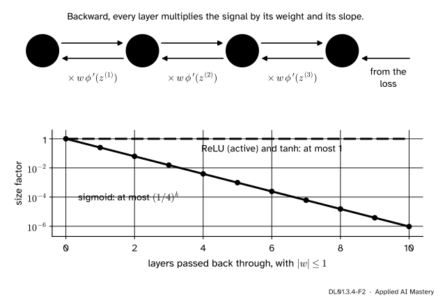
Step 3. The backward signal is a product. On the way back, every layer multiplies the gradient by its weights and by the slopes of its activation at the current pre-activations (M05.9.1). One slope per layer means a product of slopes through the depth.
DL01.3.4-F2
Backward, each layer multiplies the signal by a weight and a slope. With weights no larger than 1, a sigmoid stack loses at least a factor of 4 per layer.
Step 4. Where the slopes sit matters. A sigmoid’s slope is at most \(\tfrac14\) even in the best place. Tanh’s and an active ReLU’s are at most 1, so they can pass the signal back undiminished.
The formal statement
Use the course notation: layer \(l\) computes \({\vect{z}^{(l)} = \mat{W}^{(l)}\vect{a}^{(l-1)} + \vect{b}^{(l)}}\) and \({\vect{a}^{(l)} = \phi(\vect{z}^{(l)})}\), and \({\vect{\delta}^{(l)}}\) is the gradient of the loss with respect to \({\vect{z}^{(l)}}\). The backward rule of M05.9.2, for one example, is
Proof. Write \({\vect{u} = \mat{W}^{(l+1)\top}\vect{\delta}^{(l+1)}}\). Entry \(j\) of \({\vect{\delta}^{(l)}}\) is \({u_j\,\sigma'(z^{(l)}_j)}\), and \({0 < \sigma' \le \tfrac14}\) (DL01.3.1), so its size is at most \({\tfrac14\abs{u_j}}\). Squaring and adding over \(j\),
Take square roots. The operator norm bound of M05.9.4 gives \({\norm{\vect{u}} \le \norm{\mat{W}^{(l+1)\top}}_2\norm{\vect{\delta}^{(l+1)}}}\), and a matrix and its transpose have the same 2-norm. That is the first inequality. Applying it to layers \({l, l+1, \dots, D-1}\) in turn multiplies one factor \({\tfrac14\norm{\mat{W}^{(k)}}_2}\) per layer, which is the second. \(\square\)
With weights of size at most 1, the signal reaching layer \(l\) is at most \({4^{-(D-l)}}\) of the signal at the top: ten sigmoid layers back, at most about one millionth. Larger weights can offset the factor of 4, but they push pre-activations into the flat tails, where the slopes are far below \(\tfrac14\). Tanh’s slope is at most 1, so its factor is \({\norm{\mat{W}}_2}\) alone, and a ReLU passes the active entries unchanged. This is the vanishing gradient problem in its simplest form; DL02.4 treats it in full, with initialisation and normalisation as remedies.
Worked example
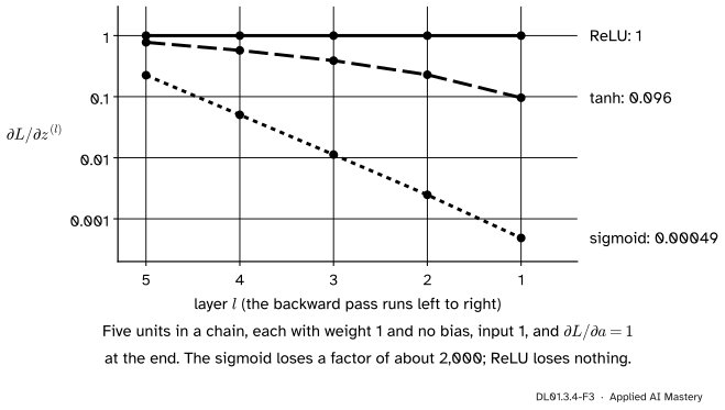
Five units in a chain. Take \({a_l = \phi(z_l)}\) with \({z_l = a_{l-1}}\) (weight 1, no bias), starting from \({a_0 = 1}\), and suppose \({\partial L/\partial a_5 = 1}\). The gradient reaching \(z_1\) is the product of the five slopes.
DL01.3.4-F3
The gradient at each layer on the way back. The sigmoid’s line falls by a factor of about 4.5 per layer.
Sigmoid. Forward, \({z_1 = 1}\), \({z_2 = \sigma(1) = 0.7311}\), \({z_3 = 0.6750}\), \({z_4 = 0.6626}\), \({z_5 = 0.6599}\). The slopes \({\sigma(z)(1 - \sigma(z))}\) at these points are \({0.1966}\), \({0.2194}\), \({0.2236}\), \({0.2244}\) and \({0.2246}\). Their product is
about \({1/2057}\), just under the bound \({4^{-5} \approx 0.00098}\).
Tanh.\({z_1 = 1}\), then \({0.7616}\), \({0.6420}\), \({0.5663}\), \({0.5126}\), with slopes \({1 - \tanh^2 z}\) of \({0.4200}\), \({0.5878}\), \({0.6793}\), \({0.7372}\) and \({0.7772}\). The product is about \({0.096}\), a loss of a factor of 10.
ReLU. Every \({z_l = 1}\), every slope is 1, and the product is 1.
Same depth, same weights, same input: the sigmoid chain delivers 200 times less signal to its first layer than the tanh chain, and about 2,000 times less than the ReLU chain.
Code
The race. The forward pass of DL01.2.2 and the batch backward pass of M05.9.2, with the hidden activation as an argument and a sigmoid output with the mean log loss. Every run starts from the same weights.
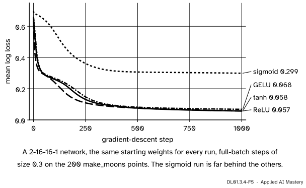
import numpy as npfrom scipy.special import erf, expitfrom sklearn.datasets import make_moonsX, y = make_moons(n_samples=200, noise=0.2, random_state=0)Phi =lambda z: 0.5* (1+ erf(z / np.sqrt(2)))ACT = { # name: (phi, phi')"sigmoid": (expit, lambda z: expit(z) * (1- expit(z))),"tanh": (np.tanh, lambda z: 1- np.tanh(z) **2),"relu": (lambda z: np.maximum(z, 0), lambda z: (z >0).astype(float)),"gelu": (lambda z: z * Phi(z), lambda z: Phi(z) + z * np.exp(-z **2/2) / np.sqrt(2* np.pi)),}def init(sizes, seed=0): rng = np.random.default_rng(seed)return [(rng.normal(0, 1/ np.sqrt(m), size=(n, m)), np.zeros(n)) for m, n inzip(sizes[:-1], sizes[1:])]def forward(layers, X, phi): Z, A = [], [X]for l, (W, b) inenumerate(layers): Z.append(A[-1] @ W.T + b) # rows are examples, W is (out, in) A.append(phi(Z[-1]) if l <len(layers) -1else expit(Z[-1]))return Z, Adef train(name, steps=1000, lr=0.3): phi, dphi = ACT[name] layers, history = init([2, 16, 16, 1]), []for step inrange(steps +1): Z, A = forward(layers, X, phi) z = Z[-1][:, 0] history.append(np.mean(np.logaddexp(0, z) - y * z)) # mean log loss, computed stablyif step == steps:break D = (A[-1] - y[:, None]) /len(y) # gradient at the output's z grads = [None] *len(layers)for l inreversed(range(len(layers))): W, b = layers[l] grads[l] = (D.T @ A[l], D.sum(axis=0))if l >0: D = (D @ W) * dphi(Z[l -1]) # the slope enters here, once per layer layers = [(W - lr * gW, b - lr * gb) for (W, b), (gW, gb) inzip(layers, grads)] accuracy = np.mean((forward(layers, X, phi)[1][-1][:, 0] >0.5) == y)return history, accuracyresults = {name: train(name) for name in ACT}for name, (h, acc) in results.items():print(f"{name:8s} loss at steps 0, 100, 300, 1000: {h[0]:.3f}{h[100]:.3f}{h[300]:.3f}{h[1000]:.3f}"f" training accuracy {acc:.1%}")
sigmoid  loss at steps 0, 100, 300, 1000: 0.699 0.566 0.335 0.299   training accuracy 86.0%
tanh     loss at steps 0, 100, 300, 1000: 0.636 0.242 0.097 0.058   training accuracy 98.5%
relu     loss at steps 0, 100, 300, 1000: 0.653 0.261 0.108 0.057   training accuracy 98.0%
gelu     loss at steps 0, 100, 300, 1000: 0.660 0.269 0.118 0.068   training accuracy 98.0%
DL01.3.4-F5
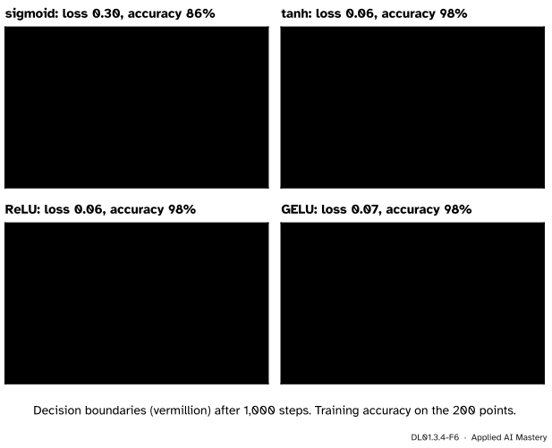
The race. Same network, same start, same steps; only the hidden activation differs. The sigmoid run is still far behind after 1,000 steps.
DL01.3.4-F6
The four decision boundaries after 1,000 steps. The sigmoid network has barely left the straight line it could draw with no hidden layer at all.
The chain of the worked example, computed:
def chain(name, depth=5): phi, dphi = ACT[name] a, slopes =1.0, []for _ inrange(depth): z = a # weight 1, no bias slopes.append(float(dphi(np.array(z)))) a =float(phi(np.array(z)))return slopes, float(np.prod(slopes))for name in ("sigmoid", "tanh", "relu"): slopes, product = chain(name)print(f"{name:8s} slopes {np.round(slopes, 4)} product {product:.2g}")
Last, scikit-learn. MLPClassifier takes the hidden activation as an argument, one of identity, logistic, tanh and relu (the default); GELU is not offered. Its default solver is Adam, met in DL02.1. To compare like with like, each run takes exactly 1,000 full-batch epochs and no early stop.
import warningsfrom sklearn.exceptions import ConvergenceWarningfrom sklearn.neural_network import MLPClassifierscores = {}for activation in ("identity", "logistic", "tanh", "relu"): model = MLPClassifier(hidden_layer_sizes=(16, 16), activation=activation, max_iter=1000, tol=0, n_iter_no_change=1000, random_state=0)with warnings.catch_warnings(): warnings.simplefilter("ignore", ConvergenceWarning) # we stop at 1,000 epochs on purpose model.fit(X, y) scores[activation] = (model.loss_, model.score(X, y))print(f"{activation:9s} final loss {model.loss_:.3f} training accuracy {model.score(X, y):.1%}")
identity  final loss 0.299   training accuracy 84.5%
logistic  final loss 0.306   training accuracy 85.0%
tanh      final loss 0.119   training accuracy 95.5%
relu      final loss 0.161   training accuracy 95.0%
The logistic network ends where the identity network does, at the loss of a straight boundary, while tanh and ReLU bend round the moons. The printed loss includes scikit-learn’s small L2 penalty (its alpha, 0.0001 by default), so it is not exactly the log loss of our own runs.
Explore
DL01.3-X1
Activation explorer
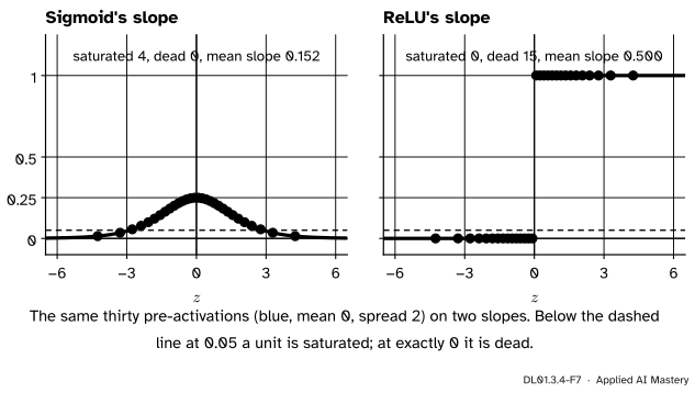
Choose an activation and set the mean and spread of thirty pre-activations. The read-out counts the units that are saturated or dead and gives the mean slope that the layer passes back.
It opens on the sigmoid with mean 0 and spread 2: 4 of the 30 units saturated, mean slope 0.152. Switch to tanh and the mean slope rises to 0.365, more than twice as much. Switch to ReLU: 15 units are dead, but the other 15 pass the signal back whole, for a mean slope of 0.5. Then move the mean to \(-2\) with spread 1 and compare ReLU, leaky ReLU, GELU and softplus.
Pitfalls
DL01.3.4-F4
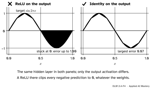
Wrong beside right. The same hidden layer feeds both outputs; a ReLU on the output cannot produce the negative half of the target at all.
“Use the same activation everywhere, output included.”
The output activation is fixed by the target, not by the hidden layers. A ReLU or a sigmoid on a regression output clips its range: no setting of the weights can predict a negative number through a ReLU. Use the identity for a real-valued target, the sigmoid for a binary one and the softmax for several classes.
“Sigmoid outputs are probabilities, so sigmoid hidden layers make the network more probabilistic.”
Hidden activations are not probabilities of anything. Sigmoid hidden units only add a factor of at most \(\tfrac14\) per layer to the backward pass. Goodfellow et al. discourage them as hidden units, and CS231n’s advice is blunter: never use the sigmoid there.
“The newest activation will fix a network that does not train.”
On the moons, tanh, ReLU and GELU end within about 0.01 of each other. A failing network is far more often failing for its learning rate, its initialisation or its data (DL01.8.3). Choose ReLU or GELU by default, check for dead or saturated units, and spend the rest of the effort elsewhere.
Check yourself
Recall
1. What output activation goes with a real-valued target, a yes-or-no target and a \(K\)-class target?
Show answer
The identity, the sigmoid and the softmax.
2. Why does a stack of sigmoid layers shrink the backward signal?
Show answer
Each layer multiplies it by the sigmoid’s slopes, which are at most \(\tfrac14\), so with weights of size at most 1 the signal shrinks by at least a factor of 4 per layer.
3. In the backward rule \(\vect{\delta}^{(l)} = {(\mat{W}^{(l+1)\top}\vect{\delta}^{(l+1)}) \odot \phi'(\vect{z}^{(l)})}\), where does the activation enter?
Show answer
Only through \({\phi'(\vect{z}^{(l)})}\), its slopes at the layer’s own pre-activations, multiplied entry by entry.
4. In the race on make_moons, which activation fell behind, and what did its boundary look like?
Show answer
The sigmoid. After 1,000 steps its loss was about 0.30 against about 0.06 for the others, and its boundary was still almost a straight line.
5. Which hidden activations does scikit-learn’s MLPClassifier offer, and which is the default?
Show answer
identity, logistic, tanh and relu; the default is relu.
Exercises
1.★ A network predicts tomorrow’s temperature change in degrees, which can be positive or negative. Its author puts a sigmoid on the output and the mean squared error as the loss. What can the network never predict, and what should the output be?
Show solution
A sigmoid outputs only numbers between 0 and 1, so the network can never predict a fall in temperature, or a rise of 1 degree or more. The target is a real number, so the output should be the identity, paired with the squared error.
2.★★ In a chain of ten tanh units with weight 1, each pre-activation is near 0.5. About how much of the signal reaches the first unit? How much with sigmoids whose pre-activations are near 0.66, as in the worked example?
Show solution
Tanh: each slope is about \({1 - \tanh^2 0.5 = 0.786}\), so \({0.786^{10} \approx 0.09}\). Sigmoid: each slope is about \({\sigma'(0.66) = 0.2246}\), so \({0.2246^{10} \approx 3.3 \times 10^{-7}}\), about a quarter of a million times less than tanh.
3.★★★ Show that for ReLU hidden layers \({\norm{\vect{\delta}^{(l)}} \le \norm{\mat{W}^{(l+1)}}_2\norm{\vect{\delta}^{(l+1)}}}\), and explain why the same bound with a factor \(\tfrac14\) cannot hold for ReLU.
Show solution
Each slope \({\operatorname{relu}'(z_j)}\) is 0 or 1, so entry \(j\) of \({\vect{\delta}^{(l)}}\) is either 0 or \(u_j\), and \({\norm{\vect{\delta}^{(l)}} \le \norm{\vect{u}} \le \norm{\mat{W}^{(l+1)}}_2\norm{\vect{\delta}^{(l+1)}}}\) as in the proof above. The factor cannot be improved: if every unit is active and \({\vect{\delta}^{(l+1)}}\) points along the top right singular vector of \({\mat{W}^{(l+1)\top}}\), then \({\vect{\delta}^{(l)} = \vect{u}}\) and \({\norm{\vect{u}} = \norm{\mat{W}^{(l+1)}}_2\norm{\vect{\delta}^{(l+1)}}}\) exactly, so no factor below 1 can hold.
Summary card
The target picks the output activation; the backward pass judges the hidden one.
DL01.3.4-F1
Output by target, hidden by choice.
Output: identity for a number, sigmoid for yes or no, softmax for \(K\) classes, each with its loss.
Backward, each layer multiplies the signal by \(\mat{W}\T\) and by the slopes \(\phi'(\vect{z})\).
A sigmoid layer multiplies its size by at most \({\tfrac14\norm{\mat{W}}_2}\).
Default hidden choice: ReLU or GELU; check for dead and saturated units.
Sources and next steps
Sources. Each was opened and checked against this lesson on 15 November 2026.
Ian Goodfellow, Yoshua Bengio and Aaron Courville, Deep Learning, chapter 6, MIT Press, 2016. Section 6.2.2 pairs output units with their costs (linear units for Gaussian outputs, sigmoid for Bernoulli, softmax for multinoulli); section 6.3 calls ReLU an excellent default and section 6.3.2 discourages sigmoid hidden units because they saturate.
Simon J. D. Prince, Understanding Deep Learning, MIT Press, 2023. The notes to chapter 3 contrast ReLU’s slope of 1 for positive inputs with the saturating slopes of sigmoid activations and survey the alternatives.
Stanford CS231n, Neural Networks Part 1: the TLDR of “Commonly used activation functions” advises ReLU with care over learning rates, never the sigmoid, and tanh only expecting it to do worse than ReLU.
scikit-learn, MLPClassifier, version 1.9.1: activation is one of identity, logistic, tanh and relu (default), the solver defaults to adam, and alpha, the L2 penalty, to 0.0001.
Next. DL01.4 pairs each output activation with its loss and derives both from maximum likelihood. DL02.4 returns to the shrinking backward signal with the tools to stop it.