A batch gradient is right on average but wrong in every single draw. Derive how its spread around the full gradient falls as 1/|B|, with the correction for sampling without replacement, measure it on the digits network, and weigh the cost of an epoch against the updates it buys.
DL01.9.3L2 Intermediate30 minIn review (what this means)
The maths and code on this page are checked by automated tests on every change, but an independent reader has not signed it off yet. Spot a mistake or a confusing step? Tell us.
Define the spread of the per-example gradients and derive that the batch gradient of |B| independent draws has expected squared error sigma^2/|B|.
State the finite-population factor (n - |B|)/(n - 1) for batches drawn without replacement and check it on four examples by hand.
Measure the spread of batch gradients on the digits network for batch sizes 1, 8, 64 and 512 and check its 1/|B| slope.
Compare batch sizes by the cost of an epoch and the number of updates it gives, and weight a short last batch by its size.
The question
A batch of 8 images costs an eighth of a batch of 64 to push through the network. Its gradient points the right way on average, but how far off is any single one? And is a batch eight times larger worth eight times the work?
From the last lesson
1. How many steps does one epoch over the 1,077 training images take with batches of 64, and how large is the last batch?
Show answer
\(\lceil 1077/64 \rceil = 17\) steps, the last of 53 images (\(1077 = {16 \cdot 64 + 53}\)).
2. What does a seeded torch.Generator passed to a DataLoader give you?
Show answer
The same sequence of shuffled epochs in every run, with a new order in each epoch.
Intuition
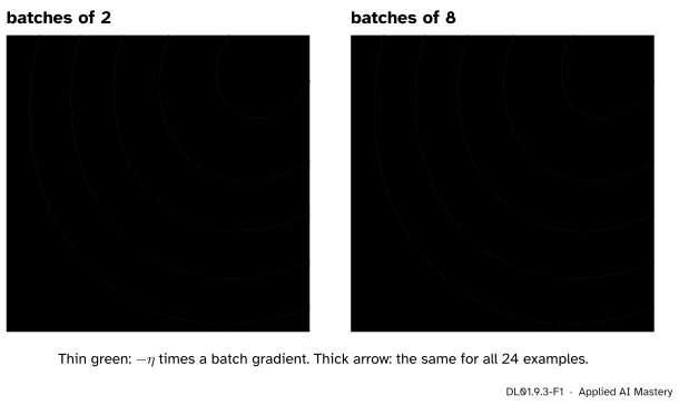
The loss of a network is a mean over the training examples, so its gradient, the full gradient\(\nabla L\), is the mean of one gradient per example. A batch gradient is the mean over only the examples in the batch. It aims at \(\nabla L\) but misses, and the picture shows by how much.
DL01.9.3-F1
Each thin green arrow is the step a batch gradient would take; the thick arrow is the full-batch step. With batches of 8 the arrows huddle around the full gradient; with batches of 2 they fan out, some pointing away from the minimum.
The batch gradients are unbiased: averaged over all possible batches they give exactly \(\nabla L\) (ML01.5.4). What changes with the batch size is their spread, and this lesson puts a number on it: four times the batch, a quarter of the spread.
Build it up
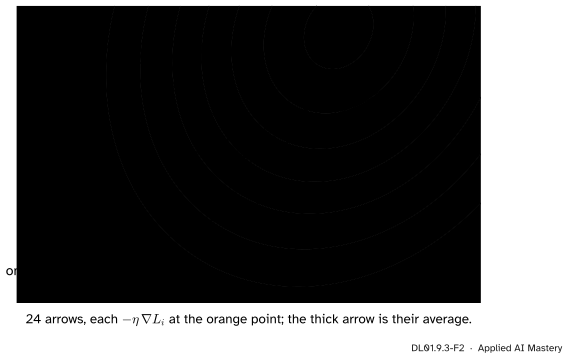
The picture uses this module’s toy problem: 24 points, a line \({wx + b}\) fitted by the mean squared error, and every gradient taken at the orange point \({(w, b)} = {(0.2, -1.0)}\).
Step 1. One gradient per example. Write \(L_i\) for the loss on example \(i\) and \(\vect{g}_i = \nabla L_i\) for its gradient. Each one points where example \(i\) alone would like the parameters to go.
DL01.9.3-F2
The 24 one-example gradients at the orange point, and their mean. Most single examples disagree with the full gradient, some strongly; their average does not.
Step 2. The full gradient is their mean.\(L = \frac{1}{n}\sum_i L_i\), and the gradient of a sum is the sum of the gradients, so \(\nabla L = \frac{1}{n} \sum_i \vect{g}_i\).
Step 3. A batch gradient is a smaller mean. For a batch \(B\) of example indices, \(\vect{g}_B = \frac{1}{\abs{B}} \sum_{i \in B} \vect{g}_i\), which is what loss.backward() computes for a mean loss over the batch.
Step 4. Measure the miss. The error of a batch gradient is the vector \({\vect{g}_B - \nabla L}\). Its squared length, averaged over the batches a loader might draw, is one number that says how noisy the step is. We call it the spread of the batch gradient.
Step 5. Measure the raw material. The same number for a batch of one, the mean squared distance of the single gradients \(\vect{g}_i\) from their mean, is the gradient variance\(\sigma^2\). Every batch size inherits its noise from it.
The formal statement
NoteDefinitions
For \(n\) examples with gradients \(\vect{g}_1, \dots, \vect{g}_n\) and mean \(\nabla L\), the gradient variance is
the sum over the parameters of the variance of each component. The spread of a batch gradient is \(\E \norm{\vect{g}_B - \nabla L}^2\), the expectation taken over the random choice of batch.
TipResult: the spread falls as \(1/\abs{B}\)
If the \(\abs{B}\) examples are drawn independently and uniformly, with replacement,
Proof for independent draws. Write \(m\) for \(\abs{B}\), to keep the lines short. Let \(I_1, \dots, I_m\) be the drawn indices and \(\vect{d}_k = {\vect{g}_{I_k} - \nabla L}\) the error of draw \(k\). Each \(I_k\) is uniform on \(1, \dots, n\), so
Take the expectation term by term. The \(m\) terms with \(k = l\) each give \(\sigma^2\). For \(k \ne l\) the draws are independent, so the expectation of the product is the product of the expectations, \({\E[\vect{d}_k] \cdot \E[\vect{d}_l]} = 0\). What is left is
Without replacement the draws of one batch are not independent: once an example is in, it cannot come again. The cross terms no longer vanish but are slightly negative, and they shrink the spread by the finite-population factor\({(n - m)/(n - 1)}\). It is close to 1 when the batch is a small part of the data and falls to 0 when \(m = n\), the full batch, which has no error at all.
Go deeper: the finite-population factor, derived
Write the batch with switches: \(s_i = 1\) if example \(i\) is in \(B\) and \(0\) if not, so that \({\vect{g}_B - \nabla L} = \frac{1}{m} \sum_i s_i \vect{e}_i\) with \(\vect{e}_i = {\vect{g}_i - \nabla L}\). The \(\vect{e}_i\) add up to zero. Every set of \(m\) distinct examples is equally likely, so
The second line is the chance that \(i\) is chosen times the chance that \(j\) is then among the other \({m - 1}\) places, filled from the remaining \({n - 1}\) examples. Write \(S\) for \(m^2\, \E \norm{\vect{g}_B - \nabla L}^2\). Expanding the square as in the main proof,
The first sum is \(n\sigma^2\). For the second, \({\sum_{i \ne j} \vect{e}_i \cdot \vect{e}_j}\) is \({\norm{\sum_i \vect{e}_i}^2 - \sum_i \norm{\vect{e}_i}^2} = {0 - n\sigma^2}\). So
and dividing by \(m^2\) gives the result. This is the variance of a sample mean under sampling without replacement, applied to each component of the gradient and added up.
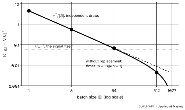
What a step costs, and what it buys. One epoch computes one gradient per example, \(n\) in all, whatever the batch size, and turns them into \(\lceil n / \abs{B} \rceil\) updates. A small batch buys many cheap, noisy steps per epoch; a large one buys few, steady ones. On the digits network (code below):
\(\abs{B}\)
Updates per epoch
Spread
1
1,077
4.45
8
135
0.552
64
17
0.0654
512
3
0.0046
The squared length of the full gradient there is about 0.056, so at \(\abs{B} = 64\) the error of a batch gradient is as large as the gradient itself.
The short last batch. With 1,077 images in batches of 64 the last batch holds 53, so its spread is larger than a full batch’s by the factor \({(64/53) \cdot (1024/1013)} \approx 1.22\). For the epoch loss, each batch’s mean loss \(L_k\) counts in proportion to its size, because \(\sum_k \abs{B_k} L_k = \sum_k \sum_{i \in B_k} L_i\) is the sum over all \(n\) examples. The epoch’s mean is therefore \(\frac{1}{n}\sum_k \abs{B_k} L_k\), the weighting of DL01.8.2; the plain average of the 17 batch means gives the short batch too much say.
Worked example
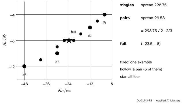
The four points of ML01, at \({(w, b)} = {(0, 0)}\). For the line \({wx + b}\) and the squared error, \(\vect{g}_i = {2 r_i (x_i, 1)}\) with residual \(r_i = {wx_i + b - y_i} = -y_i\). With \(x = 1, 2, 3, 4\) and \(y = 2, 3, 5, 6\) the four gradients are
The four one-example gradients (filled), the six pair means (hollow) and the full gradient (star). The pairs sit three times closer, in squared distance, than the singles.
The gradient variance. The errors \({\vect{g}_i - \nabla L}\) are \({(19.5, 4)}\), \({(11.5, 2)}\), \({(-6.5, -2)}\) and \({(-24.5, -4)}\). Their squared lengths are \(396.25\), \(136.25\), \(46.25\) and \(616.25\), which add up to \(1195\), so \(\sigma^2 = 1195/4 = 298.75\).
Pairs, as a loader with \(\abs{B} = 2\) draws them. The six pairs have means
Their errors from \({(-23.5, -8)}\) have squared lengths \(249.25\), \(43.25\), \(6.25\), \(6.25\), \(43.25\) and \(249.25\), which add up to \(597.5\). Every pair is equally likely, so the spread is \({597.5 / 6} \approx 99.58\).
The formula. With \(n = 4\) and \(\abs{B} = 2\): \({\frac{298.75}{2} \cdot \frac{4 - 2}{4 - 1}} = {149.375 \cdot \frac{2}{3}} \approx 99.58\). The direct count and the formula agree. Drawn independently instead, so that a pair may repeat an example, the spread would be \(298.75 / 2 = 149.375\): drawing without replacement removes a third of the noise here, because a pair is half the data.
Code
The digits network at its start and the training images of the course’s split. The gradient of every single example is written out from scratch, using the batch rules of DL01.5.
import numpy as npimport torchimport torch.nn as nnfrom sklearn.datasets import load_digitsfrom sklearn.model_selection import train_test_splittorch.manual_seed(0)torch.set_num_threads(1)digits = load_digits()X, y = digits.images.reshape(-1, 64) /16, digits.targetX_rest, _, y_rest, _ = train_test_split(X, y, test_size=0.2, stratify=y, random_state=0)X_train, _, y_train, _ = train_test_split(X_rest, y_rest, test_size=0.25, stratify=y_rest, random_state=0)n =len(y_train)model = nn.Sequential(nn.Linear(64, 32), nn.ReLU(), nn.Linear(32, 10))Xt, yt = torch.tensor(X_train, dtype=torch.float32), torch.tensor(y_train)loss = nn.CrossEntropyLoss()(model(Xt), yt)loss.backward()full = torch.cat([p.grad.reshape(-1) for p in model.parameters()]).double().numpy()def per_example_grads(model, X, y):"""One row per example: the gradient of that example's cross-entropy, parameters in model order.""" W1, b1, W2, b2 = [p.detach().double().numpy() for p in model.parameters()] Z1 = X @ W1.T + b1 A1 = np.maximum(Z1, 0.0) Z = A1 @ W2.T + b2 P = np.exp(Z - Z.max(axis=1, keepdims=True)) P /= P.sum(axis=1, keepdims=True) G = P - np.eye(10)[y] # dL_i/dz, one row per example D1 = (G @ W2) * (Z1 >0) # back through W2 and the ReLU rows =len(y)return np.hstack([np.einsum("ik,ij->ikj", D1, X).reshape(rows, -1), D1, np.einsum("ik,ij->ikj", G, A1).reshape(rows, -1), G])Gs = per_example_grads(model, X_train, y_train)sigma2 = ((Gs - Gs.mean(axis=0)) **2).sum(axis=1).mean()print(f"loss {loss.item():.3f}, {Gs.shape[1]} parameters, mean of rows = torch's gradient:", np.allclose(Gs.mean(axis=0), full, atol=1e-6))print(f"sigma^2 = {sigma2:.3f}, |full gradient|^2 = {(full **2).sum():.4f}")
loss 2.324, 2410 parameters, mean of rows = torch's gradient: True
sigma^2 = 4.449, |full gradient|^2 = 0.0562
Now draw batches as a shuffled loader does, without replacement, 400 of each size, and compare the measured spread with the formula.
gen = torch.Generator().manual_seed(0)sizes = [1, 8, 64, 512]measured, predicted = [], []for size in sizes: errors = [((Gs[torch.randperm(n, generator=gen)[:size].numpy()].mean(axis=0) - full) **2).sum()for _ inrange(400)] measured.append(np.mean(errors)) predicted.append(sigma2 / size * (n - size) / (n -1))print(f"|B| = {size:3}: measured {measured[-1]:.4f}, formula {predicted[-1]:.4f}, "f"updates per epoch {int(np.ceil(n / size))}")# Remove the finite-population factor, then fit a line to log spread against log |B|.corrected = np.array(measured) / ((n - np.array(sizes)) / (n -1))slope = np.polyfit(np.log(sizes), np.log(corrected), 1)[0]print(f"slope of log spread against log |B|: {slope:.3f}")
|B| =   1: measured 4.4699, formula 4.4489, updates per epoch 1077
|B| =   8: measured 0.5493, formula 0.5525, updates per epoch 135
|B| =  64: measured 0.0677, formula 0.0654, updates per epoch 17
|B| = 512: measured 0.0044, formula 0.0046, updates per epoch 3
slope of log spread against log |B|: -1.003
A check that the rows really are what autograd computes: one batch of 64 through PyTorch.
idx = torch.randperm(n, generator=torch.Generator().manual_seed(1))[:64]model.zero_grad()nn.CrossEntropyLoss()(model(Xt[idx]), yt[idx]).backward()batch_grad = torch.cat([p.grad.reshape(-1) for p in model.parameters()]).double().numpy()print("autograd batch gradient = mean of its rows:", np.allclose(batch_grad, Gs[idx.numpy()].mean(axis=0), atol=1e-6))print(f"short batch of 53 against full batch of 64: spread ratio {(n -53) /53/ ((n -64) /64):.3f}")
autograd batch gradient = mean of its rows: True
short batch of 53 against full batch of 64: spread ratio 1.221
DL01.9.3-F4
The spread of batch gradients on the digits network at its start. The measured points follow \(\sigma^2/\abs{B}\), a straight line of slope \(-1\) on these axes, bent down by the finite-population factor as \(\abs{B}\) approaches \(n = 1077\).
Explore
DL01.9-X1
Epoch shuffler
Twenty-four examples are tiles; set the batch size, switch shuffle and drop_last, then step through an epoch. Each batch’s step is drawn beside the full-batch step, and the read-out compares the spread so far with \({\frac{\sigma^2}{\abs{B}} \cdot \frac{n - \abs{B}}{n - 1}}\). Try sizes 1, 6 and 24, and 5 with drop_last on.
Pitfalls
DL01.9.3-F5
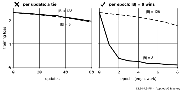
Wrong beside right. Counted in updates, batches of 8 and of 128 look alike at this learning rate. Counted in epochs, equal work, batches of 8 take 135 steps per epoch to the larger batch’s 9, and win easily.
“Doubling the batch halves the noise.”
It halves the spread, the expected squared error. The typical size of the error, its square root, falls only by a factor \(\sqrt{2}\): a batch a hundred times larger is ten times steadier for a hundred times the work per step.
“A larger batch is better, since its gradient is more accurate.”
Per step, yes; per unit of work, not necessarily. Each epoch costs \(n\) example gradients whatever the batch size, and a larger batch spends them on fewer updates. The noise of a small batch is also not pure harm: it is the “stochastic” in stochastic gradient descent. How the learning rate should move with the batch size is DL02.1.
“The short last batch is just another batch.”
Its gradient is noisier, by the factor 1.22 for 53 images against 64, and in the epoch loss its mean must count with weight \(53/1077\), not \(1/17\). Weight every batch by its size, or drop it with drop_last=True when the batch size is large and a step on a short batch would be unusually noisy.
Check yourself
Recall
1. What is the gradient variance \(\sigma^2\) of a set of examples?
Show answer
The mean squared distance of the one-example gradients from their mean, \(\sigma^2 = \frac{1}{n}\sum_i \norm{\vect{g}_i - \nabla L}^2\).
2. What is the spread of a batch gradient of \(\abs{B}\) independent draws?
Show answer
\(\sigma^2 / \abs{B}\).
3. What factor corrects it when the examples of a batch are distinct, and what is it for the full batch?
Show answer
\({(n - \abs{B})/(n - 1)}\); for \(\abs{B} = n\) it is 0, since the full batch is exact.
4. How many example gradients does one epoch cost with batches of 8, and how many with batches of 512, on 1,077 images? How many updates does each give?
Show answer
1,077 either way; 135 updates with batches of 8 and 3 with batches of 512.
5. By what factor does the typical size of the error fall when the batch grows from 8 to 512, far from the full batch?
Show answer
\(\sqrt{512/8} = \sqrt{64} = 8\), since the spread falls by 64.
Exercises
1.★ The gradient variance on the digits network is about 4.45 and \(n = 1077\). Find the spread of a batch of 32, with and without the finite-population factor.
Show solution
Without: \({4.45 / 32} \approx 0.139\). With: \({0.139 \cdot \frac{1077 - 32}{1076}} = {0.139 \cdot 0.971} \approx 0.135\). The factor matters little when the batch is 3 percent of the data.
2.★★ In the worked example, find the spread of a batch of three of the four points by the formula, and check it by listing the four possible batches.
Show solution
Formula: \({\frac{298.75}{3} \cdot \frac{4 - 3}{4 - 1}} = {99.583 \cdot \frac{1}{3}} \approx 33.19\). Listing: leaving out one point at a time, the means are \({(-30, -9.33)}\) without \(\vect{g}_1\), \({(-27.33, -8.67)}\) without \(\vect{g}_2\), \({(-21.33, -7.33)}\) without \(\vect{g}_3\) and \({(-15.33, -6.67)}\) without \(\vect{g}_4\). A batch of three that leaves out \(\vect{g}_i\) has error \({-\frac{1}{3}(\vect{g}_i - \nabla L)}\), because the four errors add up to zero. So the spread is \(\frac{1}{9}\) of the mean of the four squared errors, \({\frac{1}{9} \cdot 298.75} \approx 33.19\), as the formula says.
3.★★★ Show that, for any \(n\) and \(1 \le \abs{B} \le n\), drawing without replacement never gives a larger spread than drawing with replacement, and find the batch size at which the factor is one half.
Show solution
The ratio of the two spreads is \({(n - \abs{B})/(n - 1)}\). Since \(\abs{B} \ge 1\), the numerator is at most \({n - 1}\), so the ratio is at most 1, with equality only for \(\abs{B} = 1\), where a batch of one cannot repeat an example. Setting \({(n - \abs{B})/(n - 1)} = \frac{1}{2}\) gives \(\abs{B} = {n - \frac{n - 1}{2}} = \frac{n + 1}{2}\): about half the data. For \(n = 1077\) that is \(\abs{B} = 539\).
Summary card
A batch gradient is right on average; its spread falls as \(1/\abs{B}\).
Without replacement. Times \({(n - \abs{B})/(n - 1)}\).
Cost.\(n\) example gradients per epoch, \(\lceil n/\abs{B} \rceil\) updates.
Sources and next steps
Sources. Each was opened and checked against this lesson on 15 November 2026.
A. Zhang, Z. C. Lipton, M. Li and A. J. Smola, Dive into Deep Learning, section 12.5: averaging a minibatch of \(b\) gradients reduces the standard deviation by a factor of \(b^{-1/2}\), and beyond some point the further reduction is small compared with the linear increase in computation.
S. J. D. Prince, Understanding Deep Learning, MIT Press 2023, section 6.2: the update from a batch of indices (equation 6.10), batches drawn without replacement, epochs, and expected gradients that remain those of gradient descent.
UC Berkeley Stat 135, Lecture 3: Survey sampling, inference: for a simple random sample without replacement, the variance of the sample mean is \({\frac{\sigma^2}{n}\cdot\frac{N - n}{N - 1}}\), with \(\sigma^2\) the population variance dividing by \(N\), derived from the covariance \({-\sigma^2/(N - 1)}\) of two draws (there \(n\) is the sample and \(N\) the population).