import numpy as np

class Linear:
    """z = a W^T + b for a batch; W has shape (out, in), as in PyTorch's nn.Linear."""
    def __init__(self, W, b):
        self.W, self.b = np.array(W, float), np.array(b, float)
    def forward(self, A):
        self.A = A                                   # cache the input
        return A @ self.W.T + self.b
    def backward(self, G):
        self.dW = G.T @ self.A                       # (out, n) @ (n, in) = (out, in)
        self.db = G.sum(axis=0)                      # column sums
        return G @ self.W                            # (n, out) @ (out, in) = (n, in)
    def params(self):
        return [(self.W, "dW"), (self.b, "db")]

class ReLU:
    def forward(self, Z):
        self.mask = Z > 0
        return Z * self.mask
    def backward(self, G):
        return G * self.mask
    def params(self):
        return []

class Tanh:
    def forward(self, Z):
        self.T = np.tanh(Z)
        return self.T
    def backward(self, G):
        return G * (1 - self.T ** 2)
    def params(self):
        return []

class SoftmaxCrossEntropy:
    """Mean cross-entropy of logits Z against integer labels, fused with the softmax."""
    def forward(self, Z, labels):
        Z = Z - Z.max(axis=1, keepdims=True)
        self.P = np.exp(Z) / np.exp(Z).sum(axis=1, keepdims=True)
        self.Y = np.eye(Z.shape[1])[labels]
        return -np.mean(np.log(self.P[np.arange(len(labels)), labels]))
    def backward(self):
        return (self.P - self.Y) / len(self.P)       # the 1/n of the mean

class Sequential:
    def __init__(self, *layers):
        self.layers = layers
    def forward(self, X):
        for layer in self.layers:
            X = layer.forward(X)
        return X
    def backward(self, G):
        for layer in reversed(self.layers):
            G = layer.backward(G)
return GLayers as modules with forward and backward
Turn each layer into an object with a forward method that remembers what it needs and a backward method that returns the gradient of its input: Linear, ReLU, Tanh and a fused softmax with cross-entropy, chained by a Sequential container.
Before this lesson: DL01.5.1 One example, every number M05.7 Matrix calculus identities
What you will be able to do
- Write a layer as a module whose forward method caches what its backward method will need.
- Derive the batch gradients of a Linear layer, G-transpose A, G W and the column sums of G, by matching shapes in the course’s (out, in) convention.
- Explain where the factor 1/n in the backward of a mean loss comes from.
- Chain modules in a Sequential container, run backward in reverse order, and check every gradient for a batch of one and a batch of eight.
The question
Lesson DL01.5.1 wrote the backward pass of one network as six lines of algebra. Add a layer and the lines change; switch ReLU for tanh and they change again. Real libraries never rewrite the backward pass. How can each layer look after its own gradient, so that any stack of layers gets its backward pass for free?
From the last lesson
1. What is the gradient at the logits for a softmax output with the cross-entropy loss?
Show answer
\({\vect{p} - \vect{y}}\).
2. How does a gradient pass back through a ReLU?
Show answer
It is multiplied entry by entry by the mask \({\mathbb{I}[\vect{z} > 0]}\).
Intuition
Look at the backward pass of DL01.5.1 again. Each step used only two things: the gradient that arrived from the step after it, and something that the same layer had seen on the way forward. A dense layer needed its input; a ReLU needed to know which units were on.
So give every layer two methods. forward computes the output and keeps, in a cache, what the layer will need later. backward takes the gradient of the loss with respect to the layer’s output, returns the gradient with respect to its input, and stores the gradients of its own parameters. A layer written this way is a module.
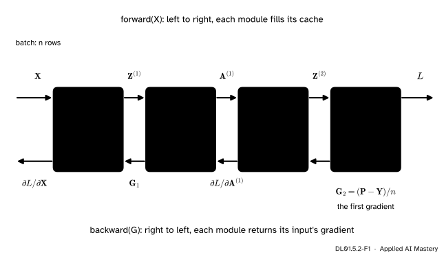
The running network as four modules. Forward carries a batch to the loss and fills each cache; backward carries gradients the other way. No module knows anything about the others.
A container then runs the modules forward in order and backward in reverse. The network is no longer six special lines; it is a list.
Build it up
Step 1. Rows are examples. A batch of \(n\) inputs is a matrix \(\mat{X}\) with one example per row. A Linear layer with weights \(\mat{W}\) of shape (out, in), the shape PyTorch’s nn.Linear stores, computes for the whole batch
\[ \mat{Z} = \mat{A}\mat{W}\T + \vect{1}\vect{b}\T , \]
where \(\mat{A}\) is its input, of shape (n, in), and \({\vect{1}\vect{b}\T}\) copies the bias into every row. Row \(i\) of this is \({(\mat{W}\vect{a}_i + \vect{b})\T}\): the one-example layer of DL01.5.1, written as a row. (M05.7.3 wrote the same layer as \({\mat{X}\mat{W}}\) with \(\mat{W}\) of shape (in, out); the gradients below are its gradients with \(\mat{W}\) transposed.)
Step 2. One gradient matrix per value. Write \(\mat{G}\) for the gradient of the loss with respect to the layer’s output \(\mat{Z}\). It has the shape of \(\mat{Z}\), (n, out): row \(i\) is the \(\vect{\delta}\) of example \(i\).
Step 3. Read the backward off the shapes. Each gradient must have the shape of the thing it is the gradient of, and each must be built from \(\mat{G}\) and one cached matrix.
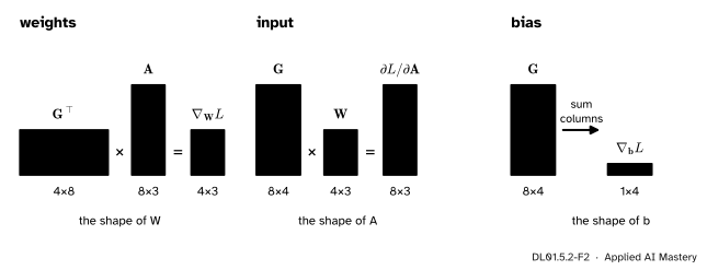
The three gradients of a Linear layer, found by matching shapes. The inner sizes must agree and the result must have the shape of the parameter or input. Only one product of the available matrices does.
Step 4. Write the modules. Linear caches \(\mat{A}\) and returns \({\mat{G}\mat{W}}\), storing \({\mat{G}\T\mat{A}}\) and the column sums of \(\mat{G}\). ReLU caches the mask and returns \({\mat{G} \odot \text{mask}}\). Tanh caches its output \(\mat{T}\) and returns \({\mat{G} \odot (1 - \mat{T} \odot \mat{T})}\), the rule of M05.9.1. The loss module comes last.
The formal statement
\({\mat{G}\T\vect{1}}\) is the vector of column sums of \(\mat{G}\).
Linear, entry by entry. \({z_{ij}} = {\sum_m a_{im} w_{jm} + b_j}\): example \(i\), output unit \(j\). The weight \(w_{jm}\) appears in \(z_{ij}\) for every example \(i\), multiplied by \(a_{im}\). Summing over those paths,
\[ \pd{L}{w_{jm}} = \sum_i g_{ij}\, a_{im} = \big(\mat{G}\T\mat{A}\big)_{jm} . \]
The bias \(b_j\) appears in every \(z_{ij}\) with coefficient 1, so its gradient is \({\sum_i g_{ij}}\), a column sum. The input \(a_{im}\) belongs to one example but feeds every output unit \(j\), so
\[ \pd{L}{a_{im}} = \sum_j g_{ij}\, w_{jm} = \big(\mat{G}\mat{W}\big)_{im} . \]
For \({n} = {1}\) these are the one-example rules of DL01.5.1, written as rows: \({\vect{\delta}\vect{a}\T}\), \(\vect{\delta}\) and \({\mat{W}\T\vect{\delta}}\).
The loss module. The batch loss is the mean \({L} = {\frac{1}{n}\sum_i \ell_i}\), where \(\ell_i\) is the cross-entropy of example \(i\). Only \(\ell_i\) depends on row \(i\) of \(\mat{Z}\), with gradient \({\vect{p}_i - \vect{y}_i}\) (DL01.5.1), and the mean multiplies it by \({1/n}\). That is the whole origin of the \(1/n\): it enters once, at the top, and every gradient below inherits it. The weight gradients then sum over the batch, so they come out as means of the one-example gradients.

What each module computes, caches and returns. Only the Linear layer has parameters; only the loss module needs the targets.
| Value | Shape | Gradient |
|---|---|---|
| \(\mat{X}\), input | (n, d) | \({\mat{G}_1\mat{W}^{(1)}}\) |
| \(\mat{W}^{(1)}\) | (h, d) | \({\mat{G}_1\T\mat{X}}\) |
| \(\mat{Z}^{(1)}\), \(\mat{A}^{(1)}\) | (n, h) | \(\mat{G}_1\), \({\mat{G}_2\mat{W}^{(2)}}\) |
| \(\mat{W}^{(2)}\) | (K, h) | \({\mat{G}_2\T\mat{A}^{(1)}}\) |
| \(\mat{Z}^{(2)}\), \(\mat{P}\) | (n, K) | \({\mat{G}_2} = {(\mat{P} - \mat{Y})/n}\) |
Here \(\mat{G}_l\) is the gradient at \(\mat{Z}^{(l)}\), and \({\mat{G}_1} = {(\mat{G}_2\mat{W}^{(2)}) \odot \text{mask}}\). For the running network \({d} = {h} = {K} = {2}\), and the batches below have \({n} = {1}\) and \({n} = {8}\).
Worked example
A batch of two, by hand: the running example \({(1, 2)}\) with class 2, and the second example of the module, \({(-1, 1)}\) with class 1, which switches hidden unit 1 off.
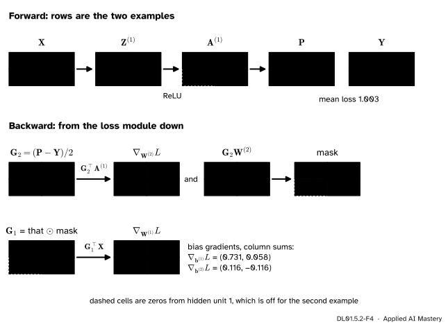
The batch of two, module by module. Each row is one example until a weight gradient sums over the rows. The dashed zeros come from the hidden unit that is off for the second example.
Forward. Row 1 is the forward pass of DL01.5.1. For row 2, \({\vect{z}^{(1)}} = {(-1 - 0.5 + 0.5,\; 0.5 + 1 - 0.5)} = {(-1, 1)}\), the mask is \({(0, 1)}\), \({\vect{a}^{(1)}} = {(0, 1)}\), the logits are \({(0.5, 0.5)}\) and \({\vect{p}} = {(0.5, 0.5)}\). The losses are 1.313 and \({\ln 2} \approx {0.693}\), with mean 1.003.
Loss module. \({\mat{G}_2} = {(\mat{P} - \mat{Y})/2}\) has rows \({(0.731, -0.731)/2} = {(0.366, -0.366)}\) and \({(0.5 - 1,\; 0.5 - 0)/2} = {(-0.25, 0.25)}\).
Linear 2. \({\nabla_{\mat{W}^{(2)}}L} = {\mat{G}_2\T\mat{A}^{(1)}}\). Its first row is \({0.366\,(0.5, 1) + (-0.25)(0, 1)} = {(0.183, 0.116)}\), and its second row is the negative. The column sums give \({\nabla_{\vect{b}^{(2)}}L} = {(0.116, -0.116)}\). The gradient passed down, \({\mat{G}_2\mat{W}^{(2)}}\), has rows \({(0.731, 0.183)}\) and \({(-0.5, -0.125)}\).
ReLU. The mask zeroes the first entry of row 2: \(\mat{G}_1\) has rows \({(0.731, 0.183)}\) and \({(0, -0.125)}\).
Linear 1. \({\nabla_{\mat{W}^{(1)}}L} = {\mat{G}_1\T\mat{X}}\). Its first row is \({0.731\,(1, 2) + 0\,(-1, 1)} = {(0.731, 1.462)}\); its second is \({0.183\,(1, 2) - 0.125\,(-1, 1)} = {(0.308, 0.241)}\). The column sums give \({\nabla_{\vect{b}^{(1)}}L} = {(0.731, 0.058)}\).
Check against DL01.5.1: the first row of \({\nabla_{\mat{W}^{(1)}}L}\) is half of \({(1.462, 2.924)}\), because the second example adds nothing to it and the mean halves the first.
Code
The modules from scratch. Each is a few lines; the container is two loops.
The running network, and a batch of one: the example of DL01.5.1.
def running(act=ReLU):
    return Sequential(Linear([[1, -0.5], [-0.5, 1]], [0.5, -0.5]), act(),
                      Linear([[1, 1], [-1, 0.5]], [-0.5, 0]))

net, loss_fn = running(), SoftmaxCrossEntropy()
loss = loss_fn.forward(net.forward(np.array([[1.0, 2.0]])), np.array([1]))
net.backward(loss_fn.backward())
lin1, lin2 = net.layers[0], net.layers[2]
print("loss", round(loss, 3), " dW1", lin1.dW.round(3).tolist(), " db2", lin2.db.round(3))
loss 1.313 dW1 [[1.462, 2.924], [0.366, 0.731]] db2 [ 0.731 -0.731]The batch of two from the worked example, then a batch of eight: the first eight points of the course’s two moons. Every gradient is checked by central differences on the batch loss.
from sklearn.datasets import make_moons

def batch_grads(net, X, labels):
    loss_fn = SoftmaxCrossEntropy()
    loss = loss_fn.forward(net.forward(X), labels)
    net.backward(loss_fn.backward())
    return loss

def worst_gap(net, X, labels, h=1e-5):
    batch_grads(net, X, labels)
    worst = 0.0
    for layer in net.layers:
        for P, name in layer.params():
            G = getattr(layer, name).copy()
            for idx in np.ndindex(P.shape):
                P[idx] += h;  up = SoftmaxCrossEntropy().forward(net.forward(X), labels)
                P[idx] -= 2 * h;  down = SoftmaxCrossEntropy().forward(net.forward(X), labels)
                P[idx] += h
                worst = max(worst, abs((up - down) / (2 * h) - G[idx]))
    return worst

X2, y2 = np.array([[1.0, 2.0], [-1.0, 1.0]]), np.array([1, 0])
net2 = running()
loss2 = batch_grads(net2, X2, y2)
print("batch of two: loss", round(loss2, 3), " dW1", net2.layers[0].dW.round(3).tolist())

X8, y8 = make_moons(n_samples=200, noise=0.2, random_state=0)
X8, y8 = X8[:8], y8[:8]
net8 = running()
loss8 = batch_grads(net8, X8, y8)
print("batch of eight: loss", round(loss8, 3), " dW1", net8.layers[0].dW.round(3).tolist())
print("largest gap to central differences:", f"{max(worst_gap(running(), X2, y2), worst_gap(running(), X8, y8)):.1e}")
batch of two: loss 1.003 dW1 [[0.731, 1.462], [0.308, 0.241]]
batch of eight: loss 2.259 dW1 [[1.457, -0.363], [0.0, 0.0]]
largest gap to central differences: 4.6e-11Look at the second row of \({\nabla_{\mat{W}^{(1)}}L}\) for the batch of eight: zeros. Hidden unit 2 is off for all eight moons points, so nothing reaches its weights: a dead unit in miniature (DL01.3.2).
The mean gradient is the average of the one-example gradients, so a loop over the eight examples, one batch of one at a time, must agree. And because the modules know nothing of each other, swapping the ReLU for a Tanh needs no new backward code.
loop = np.zeros((2, 2))
for i in range(8):
    one = running()
    batch_grads(one, X8[i:i + 1], y8[i:i + 1])
    loop += one.layers[0].dW / 8
print("mean of eight one-example gradients equals the batch gradient:", np.allclose(loop, net8.layers[0].dW))
print("tanh network, largest gap:", f"{worst_gap(running(Tanh), X8, y8):.1e}")
mean of eight one-example gradients equals the batch gradient: True
tanh network, largest gap: 1.3e-11Explore
The module’s interactive, the Backprop stepper, is in DL01.5.1. Its table is the batch-of-one version of the modules above: step to the end and compare its twelve gradients with the first code cell here. Then load the example \({(-1, 1)}\) and check that half the sum of its gradients and those of \({(1, 2)}\) gives the batch of two in the worked example.
Pitfalls
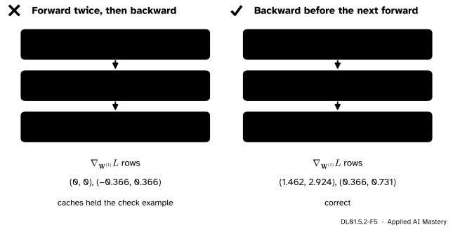
Wrong beside right. A module’s cache holds whatever it saw last. A forward call between forward and backward silently replaces the values the backward pass needs.
“Forward is a pure function, so I can call it whenever I like.”
Not in this design: forward also fills the cache. Run a check example through the network between the training forward and the backward, and the Linear layers multiply the training gradient by the check example’s inputs. Here \({\nabla_{\mat{W}^{(1)}}L}\) comes out with rows \({(0, 0)}\) and \({(-0.366, 0.366)}\) instead of \({(1.462, 2.924)}\) and \({(0.366, 0.731)}\), with no error raised. Finish backward first.
“The loss is a mean, so I divide the weight gradients by n at the end.”
The \(1/n\) is already in \({(\mat{P} - \mat{Y})/n}\), and every gradient below inherits it. Dividing again gives gradients \(n\) times too small, which looks exactly like a learning rate \(n\) times too small: training is slow, not broken, so the bug survives for a long time. A gradient check on a batch of more than one example catches it.
“Bias gradients have the shape of G.”
\(\mat{G}\) is (n, out) but \(\vect{b}\) is (out,). The bias was copied into every row on the way forward, so its gradient sums over the rows on the way back. Forgetting the sum gives an array of the wrong shape, and NumPy’s broadcasting may even let the update run.
Check yourself
Recall
1. What does a module’s forward method do besides computing its output?
Show answer
It caches what its backward method will need: the input for Linear, the mask for ReLU, the output for Tanh, the probabilities and targets for the loss.
2. Give the three gradients of a Linear layer for a batch, in the course’s (out, in) convention.
Show answer
\({\nabla_{\mat{W}}L} = {\mat{G}\T\mat{A}}\), \({\nabla_{\vect{b}}L}\) = the column sums of \(\mat{G}\), and \({\partial L/\partial\mat{A}} = {\mat{G}\mat{W}}\).
3. What does the fused softmax-cross-entropy module return from backward, and why the \(1/n\)?
Show answer
\({(\mat{P} - \mat{Y})/n}\). The loss is the mean of \(n\) per-example losses, so each example’s gradient is multiplied by \(1/n\).
4. In what order does a Sequential container call backward?
Show answer
In reverse: the last module first, each one handing its returned gradient to the module before it.
5. Why is the second row of \({\nabla_{\mat{W}^{(1)}}L}\) zero for the batch of eight moons points?
Show answer
Hidden unit 2 is off for all eight examples, so the ReLU mask zeroes its column of \(\mat{G}_1\), and every gradient that reaches its weights is zero.
Exercises
1. ★ A Linear layer maps 64 inputs to 32 outputs on a batch of 100. Give the shapes of \(\mat{A}\), \(\mat{W}\), \(\mat{G}\), \({\mat{G}\T\mat{A}}\), \({\mat{G}\mat{W}}\) and the bias gradient.
Show solution
\(\mat{A}\) is (100, 64), \(\mat{W}\) is (32, 64) and \(\mat{G}\) is (100, 32), the shape of the output. \({\mat{G}\T\mat{A}}\) is \({(32, 100)(100, 64)} = {(32, 64)}\), the shape of \(\mat{W}\); \({\mat{G}\mat{W}}\) is \({(100, 32)(32, 64)} = {(100, 64)}\), the shape of \(\mat{A}\); and the bias gradient is the 32 column sums of \(\mat{G}\).
2. ★★ Write the forward and backward of a Sigmoid module that caches as little as possible, and use it to find the gradient passed back for \({\mat{Z}} = {[[0, \ln 3]]}\) and \({\mat{G}} = {[[4, 4]]}\).
Show solution
Forward computes \({\mat{S}} = {\sigma(\mat{Z})}\) and caches \(\mat{S}\) alone, because \({\sigma'(z)} = {\sigma(z)(1 - \sigma(z))}\) (DL01.3.1) needs only the output. Backward returns \({\mat{G} \odot \mat{S} \odot (1 - \mat{S})}\). Here \({\sigma(0)} = {0.5}\) and \({\sigma(\ln 3)} = {3/(1 + 3)} = {0.75}\), so the result is one row with entries \({4 \times 0.5 \times 0.5} = {1}\) and \({4 \times 0.75 \times 0.25} = {0.75}\).
3. ★★★ Show that the bias gradient \({\mat{G}\T\vect{1}}\) is what you get by treating the bias as an extra weight on an input that is always 1: append a column of ones to \(\mat{A}\) and the column \(\vect{b}\) to \(\mat{W}\), and apply \({\mat{G}\T\mat{A}}\).
Show solution
Let \({\tilde{\mat{A}}} = {[\mat{A} \;\; \vect{1}]}\), of shape (n, in + 1), and \({\tilde{\mat{W}}} = {[\mat{W} \;\; \vect{b}]}\), of shape (out, in + 1). Then \({\tilde{\mat{A}}\tilde{\mat{W}}\T} = {\mat{A}\mat{W}\T + \vect{1}\vect{b}\T}\), the same layer. Its weight gradient is \({\mat{G}\T\tilde{\mat{A}}} = {[\mat{G}\T\mat{A} \;\; \mat{G}\T\vect{1}]}\). The columns that belong to the inputs are \({\nabla_{\mat{W}}L}\), and the last column, the gradient of the weight that plays the bias, is \({\mat{G}\T\vect{1}}\): the column sums of \(\mat{G}\).
Summary card
A module caches on the way forward and returns its input’s gradient on the way back.
Forward fills caches; backward empties them.
- Linear: \({\nabla_{\mat{W}}L} = {\mat{G}\T\mat{A}}\), bias: column sums, input: \({\mat{G}\mat{W}}\).
- ReLU: \({\mat{G} \odot \text{mask}}\). Tanh: \({\mat{G} \odot (1 - \mat{T}^{\odot 2})}\).
- Softmax with mean cross-entropy: \({(\mat{P} - \mat{Y})/n}\).
- Sequential: forward in order, backward in reverse.
Sources and next steps
Sources. Each was opened and checked against this lesson on 15 November 2026.
- S. J. D. Prince, Understanding Deep Learning (MIT Press, 2023), section 7.4.2: each functional component, such as a linear transform, a ReLU or a loss, knows how to compute its own derivative, and the framework knows the order of the operations; for a batch, the first dimension of the input indexes the batch element.
- Stanford CS231n, Backpropagation, Intuitions. “Modularity: Sigmoid example”: any differentiable function can act as a gate, and gates can be grouped; the section on vectorised operations finds the gradients of a matrix product by dimension analysis.
- A. Zhang, Z. C. Lipton, M. Li and A. J. Smola, Dive into Deep Learning, section 5.3: backpropagation reuses the intermediate values stored by forward propagation, which must be kept until backpropagation is complete, one reason training needs more memory than prediction.
- PyTorch 2.15 documentation,
torch.nn.Linear: the layer computes \({y = xA\T + b}\), and its weight has shape (out_features, in_features).
Next. DL01.5.3 Branches, sums and shared weights leaves the straight chain: values that feed two places, skips, and weights used twice.
This lesson unlocks
DL01.5.3 Branches, sums and shared weights
Your progress is saved in this browser only. No account, no tracking.