Open the trained network up: its 32 first-layer weight vectors drawn as images and its hidden activations projected with PCA. Then shuffle the pixels of every image the same way, retrain, and see accuracy stay put, which proves the network never used which pixels are neighbours.
DL01.10.4L2 Intermediate25 minIn review (what this means)
The maths and code on this page are checked by automated tests on every change, but an independent reader has not signed it off yet. Spot a mistake or a confusing step? Tell us.
Draw a first-layer weight vector as an image and read which pixels push a hidden unit up or down.
Project hidden activations to two dimensions with PCA and say what such a picture can and cannot show.
Prove that shuffling the input pixels and the columns of the first weight matrix the same way leaves a multilayer perceptron’s outputs and its training unchanged.
Write a one-page project report: question, data, method, result and limits.
The question
The network reads these digits about 97 percent of the time. Does it see strokes and loops, the way you do? Here is a test: shuffle the 64 pixels of every image in one fixed way, so that the digits turn into noise to your eye, and train again. What happens to its accuracy?
From the last lesson
1. What is the network’s test accuracy, with its standard error?
Show answer
349 of 360, 96.9 percent, standard error 0.9 points.
2. Is the network shown to be better than logistic regression on the test set?
Show answer
No. The gap is 2 images in 360, 0.56 points, smaller than its paired standard error of 0.68 points.
Intuition
Each hidden unit of the network starts with a weighted sum of the 64 pixels: one weight per pixel. Nothing in that sum knows that pixel 10 sits beside pixel 11, or above pixel 18. Reorder the pixels and reorder the weights the same way, and every sum is unchanged: the same products, added in a different order.
DL01.10.4-F1
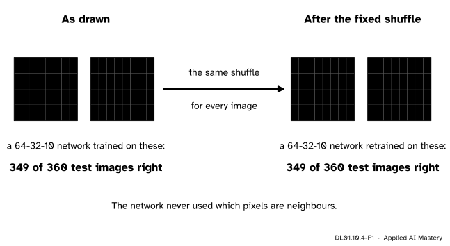
One fixed shuffle of the pixels makes the digits unreadable to a person. A network retrained on shuffled images scores just as well: it never relied on which pixels are neighbours.
So the shuffle costs the network nothing it was using. That is not a weakness of this training run; it is built into the architecture. A multilayer perceptron treats an image as a list of 64 unrelated numbers. It succeeds here because the digits are small, centred and scaled to the same size. Convolutional networks (DL03) are built to use what the perceptron ignores: that nearby pixels belong together, and that a stroke means the same thing wherever it appears.
Build it up
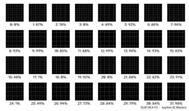
Step 1. The weights as pictures. Unit \(i\) of the hidden layer computes \({z_i = \vect{w}_i \cdot \vect{x} + b_i}\) with one weight per pixel. Put the 64 weights back on the 8 by 8 grid and the unit becomes a picture: orange where ink raises \(z_i\), grey where ink lowers it.
DL01.10.4-F2
The 32 first-layer weight vectors as images. Under each: the share of the training images on which that unit is active (its pre-activation is above zero).
A few units look like parts of digits, a band or a curve. Most are blotchy: a unit is a direction in the space of 64 pixels that is useful to the output layer, not a template a person would draw. The shares tell another story. Six units are active on fewer than 1 percent of the training images, and one, unit 20, on none at all: a dead unit (DL01.3.2), which passes back no gradient and can no longer learn. The network does its work with about 26 units.
Step 2. The hidden layer as a new description. For each image the 32 activations are a new set of features, learned for the job. To glimpse them, project the 32 numbers of each test image onto the two directions of largest variance with PCA, used here as a tool (its theory is M03.6).
DL01.10.4-F3
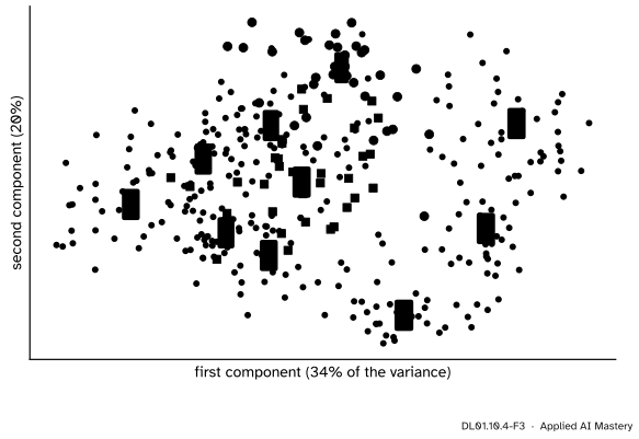
The hidden activations of the test images, projected on their first two principal components. The ones (blue circles) and the eights (sky-blue squares) are picked out.
Classes gather in regions: 0 at the bottom, 4 and 6 on the right, the ones at the top. Others, 7, 8, 9 and 5, crowd the middle. This flat view keeps only 54 percent of the variance of the 32 numbers; in all 32 dimensions the output layer separates the classes well enough for 97 percent accuracy.
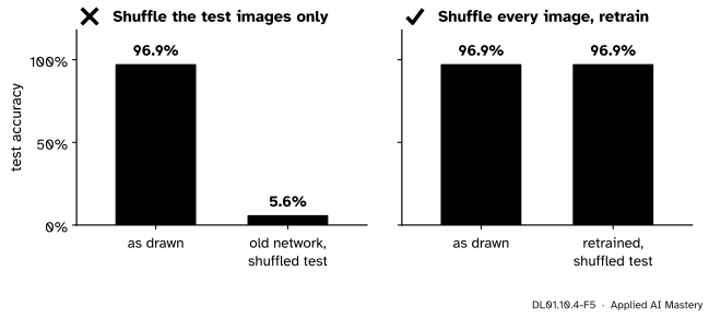
Step 3. Shuffle and retrain. Draw one random order of the 64 positions, perm = torch.randperm(64) from a generator seeded with 0, and replace every image \(\vect{x}\) by x[perm]. Retrain from the usual seed. The shuffled network gets 349 of 360 test images right, the same count as the original, and 352 validation images against 351.
Step 4. The old network on shuffled images. Give the original network the shuffled test images and it gets 20 of 360 right, 5.6 percent: worse than always answering one class. Its weights belong to pixel positions, and the shuffle moved the pixels away from them.
The formal statement
Write the shuffle as a permutation matrix\(\mat{P}\): row \(i\) of \(\mat{P}\) is \(\vect{e}_{\pi(i)}\T\), so \({(\mat{P}\vect{x})_i = x_{\pi(i)}}\), where \(\pi\) is perm. A permutation matrix satisfies \({\mat{P}\T\mat{P} = \mat{I}}\): column \(j\) of \(\mat{P}\) has a single 1, so the dot product of two columns is 1 when they are the same column and 0 otherwise.
NoteShuffling the pixels changes nothing an MLP can use
Let a network have first-layer weights \(\mat{W}\) and any other parameters \(\theta\). Give a second network the weights \({\mat{W}' = \mat{W}\mat{P}\T}\) and the same \(\theta\). Then:
On shuffled inputs it computes exactly what the first computes on the originals.
Trained by SGD on the shuffled images with the same batches, it stays at \({\mat{W}'_t = \mat{W}_t\mat{P}\T}\) after every step \(t\).
Proof of 1. The first layer’s pre-activation on a shuffled input is
and everything after the first layer is shared, so the outputs, the losses and all the gradients with respect to later layers are equal.
Proof of 2, by induction. Suppose \({\mat{W}'_t = \mat{W}_t\mat{P}\T}\) before a step. By part 1 both networks have the same pre-activations, hence the same \(\vect{\delta}^{(1)}\), the gradient of the loss with respect to them. For one example the weight gradient is \(\vect{\delta}^{(1)}\) times the input transposed (M05.9), so for the shuffled network
while every other parameter takes the same step in both networks. ∎
In code, \({\mat{W}\mat{P}\T}\) is W[:, perm]: column \(i\) of the new matrix is column \(\pi(i)\) of the old one, the weight that belonged to the pixel now sitting at position \(i\).
Why a fresh start does just as well. PyTorch draws every first-layer weight independently from the same uniform distribution. Permuting the columns of such a matrix gives a matrix with exactly the same distribution. So training on shuffled images from a fresh random start is, in distribution, the same experiment as training on the originals: the expected accuracy is identical, and only the luck of the particular start differs. That is what the code finds: 349 against 349 on test, 352 against 351 on validation.
Worked example
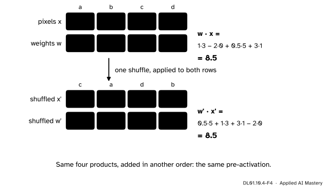
A four-pixel image \({\vect{x} = (3, 0, 5, 1)}\) and one hidden unit with weights \({\vect{w} = (1, -2, 0.5, 3)}\) give
Shuffle with \({\pi = (3, 1, 4, 2)}\), counting from 1: the new image takes pixels 3, 1, 4 and 2 in that order, \({\vect{x}' = (5, 3, 1, 0)}\). Shuffle the weights the same way, \({\vect{w}' = (0.5, 1, 3, -2)}\). Then
The proof in miniature: each weight still meets its own pixel, so the four products are the same.
Each weight still meets the pixel it met before; only the order of the four products changed. With the original weights \(\vect{w}\) on the shuffled image, though, the sum is \({1 \cdot 5 - 2 \cdot 3 + 0.5 \cdot 1 + 3 \cdot 0 = -0.5}\): the old network on shuffled pixels computes something else entirely.
Code
The data and the training function of DL01.10.3, now with an optional shuffle and an optional starting point.
What the first layer holds, and how often each unit is active on the training images.
W = model[0].weight.detach()with torch.no_grad(): H_train = model[1](model[0](X_train)) H_test = model[1](model[0](X_test)).numpy()share = (H_train >0).float().mean(dim=0)print("weight images:", tuple(W.reshape(32, 8, 8).shape))print("units active on no training image:", torch.nonzero(share ==0).flatten().tolist())print("units active on under 1 percent:", int((share <0.01).sum()))print(f"active units per test image, on average: {(H_test >0).sum(axis=1).mean():.1f} of 32")pca = PCA(n_components=2).fit(H_test)print("variance kept by two components:", pca.explained_variance_ratio_.round(3))
weight images: (32, 8, 8)
units active on no training image: [20]
units active on under 1 percent: 6
active units per test image, on average: 22.4 of 32
variance kept by two components: [0.338 0.201]
The shuffle experiment: retrain from a fresh start, and try the old network on shuffled images.
retrained on shuffled pixels: validation 352  test 349
original network, shuffled test images: 20 of 360
The theorem, checked: start the shuffled network from the original’s starting weights with the columns of \(\mat{W}\) shuffled, W[:, perm], and compare the two runs step by step.
torch.manual_seed(0)start = nn.Sequential(nn.Linear(64, 32), nn.ReLU(), nn.Linear(32, 10)).state_dict()start = {name: value.clone() for name, value in start.items()}start["0.weight"] = start["0.weight"][:, perm]matched, losses_matched = train_kept(perm=perm, init=start)_, losses_plain = train_kept()loss_gap =max(abs(a - b) for a, b inzip(losses_plain, losses_matched))weight_gap = (matched[0].weight - model[0].weight[:, perm]).abs().max().item()print(f"{len(losses_plain)} steps; largest difference in a batch loss {loss_gap:.1e}, "f"in a first-layer weight {weight_gap:.1e}")
1020 steps; largest difference in a batch loss 2.4e-07, in a first-layer weight 6.6e-07
The two runs agree to about seven digits over 1,020 steps, the precision of float32: the products are the same, but added in a different order, which rounds differently in the last bit. The theorem holds exactly in exact arithmetic.
The other side of the coin: move every test image one column to the left, a change a person would hardly notice.
def shift_left(X):"""Move each image one column left; the right-hand column becomes blank.""" images = X.reshape(-1, 8, 8)return torch.cat([images[:, :, 1:], torch.zeros(len(X), 8, 1)], dim=2).reshape(-1, 64)ones = y_test ==1print("test ones read as 1:", right(model, X_test[ones], y_test[ones])," after the shift:", right(model, shift_left(X_test[ones]), y_test[ones]), "of", int(ones.sum()))print("all test images after the shift:", right(model, shift_left(X_test), y_test), "of 360")
test ones read as 1: 35  after the shift: 12 of 36
all test images after the shift: 167 of 360
Only 12 of the 36 ones survive the shift, and the whole test set falls from 349 to 167 right. Each weight belongs to one pixel position, so a stroke one column over meets different weights.
Explore
DL01.10-X1
Digit sketchpad
Paint a digit on the 8 by 8 pad, or press Next test image, and watch the ten probabilities and the 32 hidden activations of the network trained in this module. Then choose Shuffled: retrained network: the input turns to noise, yet the answer barely moves. Choose Shuffled: original network to see the first network lost on the same noise.
The sketchpad’s networks are the ones trained above, their weights rounded to four decimals and stored in the page. Try painting a 1 one column to the left of where the test images put it: as the last cell of the code showed, the network often reads it as something else, because a perceptron has no way to know that a shifted stroke is the same stroke.
Pitfalls
DL01.10.4-F5
Wrong beside right. Shuffling only the test images measures the wrong thing; the claim is about a network trained on shuffled images.
“Shuffling the pixels breaks the network: accuracy falls to 5.6 percent.”
That is the old network meeting images it was never trained on, a mismatch between training and test data. The statement that matters is about the architecture: retrained on shuffled images, the same network design does exactly as well.
“Each weight image is the template of one digit.”
A hidden unit feeds all ten logits through its column of \(\mat{W}^{(2)}\), with positive weight to some classes and negative to others. Its picture shows what raises it, not which class it votes for.
“In the PCA picture 7, 8 and 9 overlap, so the network must confuse them.”
Two components keep 54 percent of the variance of 32 numbers. Points that overlap in a projection can be far apart in the full space; judge confusion by the confusion matrix, not by the projection.
“An MLP ignores where pixels are, so it is useless for images.”
On these small, centred, size-normalised digits it scores 97 percent. Its weakness shows when the same pattern can appear in different places or the images are large: it must learn each position separately, with a weight for every pixel of every unit. That is the problem DL03 solves.
Check yourself
Recall
1. What does a first-layer weight vector drawn as an 8 by 8 image show?
Show answer
Which pixels raise the unit’s pre-activation when inked (positive weights) and which lower it (negative weights).
2. Why does \({\mat{W}\mat{P}\T\mat{P}\vect{x} = \mat{W}\vect{x}}\)?
Show answer
Because a permutation matrix satisfies \({\mat{P}\T\mat{P} = \mat{I}}\).
3. How is \({\mat{W}\mat{P}\T}\) written in PyTorch, for a shuffle perm?
Show answer
W[:, perm]: the columns of \(\mat{W}\) reordered by perm.
4. Why does a network trained on shuffled images from a fresh random start do as well as one trained on the originals?
Show answer
The first-layer weights start independent and identically distributed, so their shuffled columns have the same distribution; by the theorem the two experiments are then the same in distribution.
5. What share of the variance of the hidden activations do two principal components keep here?
Show answer
About 54 percent: 34 percent for the first and 20 percent for the second.
Exercises
1.★ Shuffle \({\vect{x} = (2, 7, 0, 4)}\) with \({\pi = (4, 3, 1, 2)}\), counting from 1, and the weights \({\vect{w} = (1, 0, -1, 2)}\) the same way. Check that the dot product is unchanged, and compute what the unshuffled weights give on the shuffled image.
2.★★ Show that \({\mat{P}\T\mat{P} = \mat{I}}\) for the permutation matrix of \({\pi = (2, 3, 1)}\), and that \({\mat{P}\vect{x}}\) is \({(x_2, x_3, x_1)}\).
Show solution
Row \(i\) of \(\mat{P}\) is \(\vect{e}_{\pi(i)}\T\), so the rows are \(\vect{e}_2\T\), \(\vect{e}_3\T\) and \(\vect{e}_1\T\):
Then \({\mat{P}\vect{x} = (x_2, x_3, x_1)}\). Entry \({(j, k)}\) of \({\mat{P}\T\mat{P}}\) is the dot product of columns \(j\) and \(k\) of \(\mat{P}\). Each column holds a single 1, in a different row for each column, so the dot product is 1 when \({j = k}\) and 0 otherwise: \({\mat{P}\T\mat{P} = \mat{I}}\).
3.★★★ A one-dimensional convolution with kernel \({(k_1, k_2)}\) maps an input \({(x_1, \dots, x_4)}\) to \({y_i = k_1 x_i + k_2 x_{i+1}}\) for \({i = 1, 2, 3}\). Write it as a 3 by 4 matrix, and explain why, for a typical shuffle, no kernel can do on shuffled inputs what this one does on the originals, although an unconstrained matrix could.
Show solution
The matrix has rows \({(k_1, k_2, 0, 0)}\), \({(0, k_1, k_2, 0)}\) and \({(0, 0, k_1, k_2)}\): the same two numbers on neighbouring positions in every row. On shuffled inputs the matching weights would be \({\mat{K}\mat{P}\T}\), whose columns are reordered, so the two numbers no longer sit side by side in each row and the rows are no longer shifted copies of one another (unless the shuffle happens to keep every pair of neighbours together and in order). A convolution can only produce matrices of the banded, shifted form, so it cannot represent \({\mat{K}\mat{P}\T}\); a fully connected layer can represent any matrix, which is exactly why the shuffle costs it nothing, and also why it has to learn every position separately.
Summary card
The one-page write-up
Question. Can a small multilayer perceptron classify 8 by 8 handwritten digits better than logistic regression on the pixels?
Data. scikit-learn’s load_digits: 1,797 images, ten balanced classes, pixels 0 to 16 divided by 16. Stratified split: 1,077 training, 360 validation, 360 test images (DL01.9.4).
Method. A 64-32-10 ReLU network, cross-entropy, SGD with batches of 32 for 30 epochs, keeping the epoch with the lowest validation loss. Width and learning rate chosen from a 3 by 3 grid with the one-standard-error rule on validation accuracy. Checks first: starting loss 2.32, one batch fitted.
Result. 349 of 360 test images right, 96.9 percent with a standard error of 0.9 points, against 96.4 percent for logistic regression: a gap of 0.56 points with a paired standard error of 0.68, so no evidence of a difference. Mistakes are scattered; eights called ones and fours called eights are the most common.
Limits. One split and one seed; 360 test images cannot separate models closer than about one point. The images come from the 13 writers of the UCI test part and the split mixes each writer’s digits, so the score measures reading these writers, not new ones. The network ignores which pixels are neighbours (retrained on shuffled pixels it scores the same), so it would not cope with shifted or larger images: the task for convolutions.
An MLP sees a list of numbers, not a picture.
DL01.10.4-F1
Shuffle the pixels, retrain, same accuracy.
Weight image: the 64 weights of a unit on the 8 by 8 grid.
\({\mat{W}\mat{P}\T \cdot \mat{P}\vect{x} = \mat{W}\vect{x}}\), since \({\mat{P}\T\mat{P} = \mat{I}}\); in code W[:, perm].
SGD keeps \({\mat{W}'_t = \mat{W}_t\mat{P}\T}\), so shuffled training is the same experiment.
Old network on shuffled images: 20 of 360. Retrained: 349 of 360.
Sources and next steps
Sources. Each was opened and checked against this lesson on 15 November 2026.
Cristian Ivan, Convolutional neural networks on randomized data, CVPR Workshops 2019. Section 2.1: an MLP trained on natural and on pixel-wise permuted MNIST images performs almost identically, while a CNN trained on permuted images learns later and scores consistently lower; section 2.3 calls the MLP invariant under this transformation.
scikit-learn 1.9 API reference, PCA: linear dimensionality reduction by the singular value decomposition of the data, which is centred but not scaled; explained_variance_ratio_ holds the share of variance of each component.
PyTorch 2.15 documentation, torch.nn.Linear: every weight starts independently uniform on \({(-\sqrt{k}, \sqrt{k})}\) with k = 1/in_features, the fact behind the argument that a fresh start on shuffled images is the same experiment.
Next. DL02, Training deep networks, takes this loop further: better optimisers, schedules, initialisation and regularisation. DL03, Convolutional networks, builds the layer that uses what this network cannot see.