Build the 64-32-10 network, run the two first checks before trusting the loop, train it with the fit function of DL01.8.4, and choose the width and learning rate from a grid of nine runs using the validation set alone, with the one-standard-error rule.
DL01.10.2L2 Intermediate25 minIn review (what this means)
The maths and code on this page are checked by automated tests on every change, but an independent reader has not signed it off yet. Spot a mistake or a confusing step? Tell us.
Count the parameters of a 64-H-10 network and the updates in a run of E epochs with batches of B.
Run the two first checks on a new training loop: a starting loss near ln 10, and one batch driven to nearly zero.
Train the network with DataLoader, nn.CrossEntropyLoss, torch.optim.SGD and the fit function, keeping the best epoch’s weights.
Choose a width and a learning rate from a small grid with the one-standard-error rule, using the validation set only.
The question
You have a network design, a loader and a fit function. Before you spend any time training: how do you know the loop works at all? And when nine combinations of width and learning rate give validation scores within a few images of each other, which one do you keep?
From the last lesson
1. What validation accuracy must the network beat, and where does that number come from?
Show answer
96.7 percent (348 of 360): logistic regression on the pixels divided by 16, fitted on the training images and scored on the validation images.
2. Write accuracy in terms of the per-class recalls.
Show answer
\({A = \sum_k (n_k/n)\, R_k}\), the recalls weighted by the class shares.
Intuition
Training a network for a real task is the same loop as DL01.8, wrapped in two habits. Check before you trust: two quick tests catch most broken set-ups in seconds. Choose with the validation set only: every decision, from the epoch to keep to the width of the hidden layer, is made on the 360 validation images, and the test images stay closed.
DL01.10.2-F1
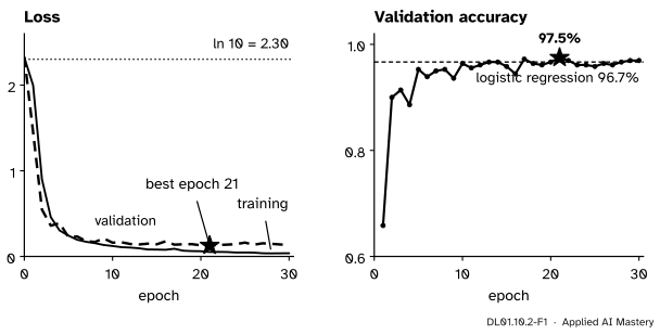
The chosen network’s run. The loss starts at \(\ln 10\), as it must, and the weights of epoch 21, with the lowest validation loss, are kept: 97.5 percent on validation, just above the baseline.
Read the picture from left to right. The loss starts at about 2.30, the loss of a network that spreads its belief evenly over ten classes. Within five epochs it has fallen below 0.3. After epoch 21 the validation loss stops improving, so the fit function keeps that epoch’s weights. On the right, those weights get 351 of 360 validation images right: three more than the baseline.
Build it up
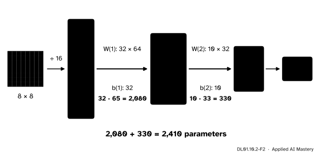
Step 1. The network. 64 inputs, one hidden layer of 32 ReLU units, 10 outputs: the logits. A layer from \(n_{\text{in}}\) to \(n_{\text{out}}\) has \({n_{\text{out}}(n_{\text{in}} + 1)}\) parameters (DL01.1.3), so the two layers have \({32 \cdot 65 = 2{,}080}\) and \({10 \cdot 33 = 330}\), together 2,410.
DL01.10.2-F2
The project network. Weights are stored with shape (out, in), as nn.Linear keeps them.
Step 2. The loaders. The training images go into a DataLoader with batches of 32, shuffled each epoch by a generator seeded with 0 (DL01.9.2). One epoch is \({\lceil 1077 / 32 \rceil = 34}\) steps: 33 full batches and a last one of 21 images.
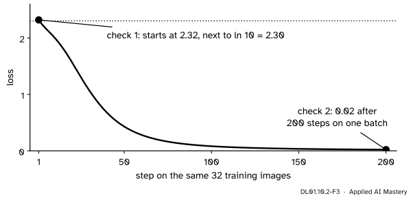
Step 3. Check 1: the starting loss. A freshly built network has small random weights, so its logits are all near zero and its probabilities near \({1/10}\) each. The loss should start near \({\ln 10 \approx 2.303}\). Ours starts at 2.324.
Step 4. Check 2: one batch, overfitted. Train on the same 32 images again and again. A working loop drives their loss towards zero, because 2,410 parameters can memorise 32 images. Ours goes from 2.32 to 0.02 in 200 steps. If either check fails, nothing after it can be trusted (DL01.8.3).
DL01.10.2-F3
The two first checks on one picture: the right starting loss, and a batch the loop can memorise.
Step 5. Train. The fit function of DL01.8.4 runs 30 epochs of nn.CrossEntropyLoss and plain torch.optim.SGD, evaluates on the validation loader after every epoch, and keeps the weights of the epoch with the lowest validation loss.
Step 6. The grid. Three widths (16, 32 and 64 hidden units) and three learning rates (0.03, 0.1 and 0.3) make nine runs of a fraction of a second each. Each is scored by the validation accuracy of its kept weights.
The formal statement
Why the start is \(\ln 10\). For one image with label \(y\) and logits \(\vect{z}\), the loss is \({-z_y + \ln \sum_k e^{z_k}}\) (DL01.4.3). If every logit equals the same number \(c\),
So any network whose logits start nearly equal starts near \(\ln 10\). A start far above it, as in this lesson’s pitfall, means logits that are already large and confidently wrong.
Counting the work. With \(n\) training images, batches of \(B\) and \(E\) epochs, the run makes \({E \lceil n/B \rceil}\) updates: here \({30 \cdot 34 = 1{,}020}\).
Choosing from the grid. A validation accuracy measured on \(n\) images is itself uncertain. If the best run gets \(a^*\) of \(n\) right, its standard error in images is
the spread we would see from one validation set of \(n\) images to another (it is derived in DL01.10.3 from the standard error of ML01.2.3). Two runs closer than \(s\) are not reliably different.
NoteThe one-standard-error rule
Among the runs whose validation count is at least \({a^* - s}\), keep the one with the fewest parameters; between runs of the same size, keep the higher count.
The rule never looks at the test images and it prefers the simpler model when the data cannot tell two apart. It is a common rule of thumb for choosing by validation, not a theorem; scikit-learn’s documentation states the same rule for cross-validated scores, citing Hastie, Tibshirani and Friedman. Here it is applied to the standard error of one validation set.
Worked example
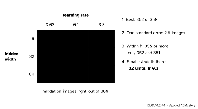
The nine runs, as validation images right out of 360:
DL01.10.2-F4
The grid and the rule. Two runs lie within one standard error of the best; the smaller one is kept.
The best is 352, from width 64 and learning rate 0.3: \({p^* = 352/360 = 0.9778}\).
Then \({1 - p^* = 0.0222}\), and the product \({p^*(1 - p^*)}\) is 0.02173; divided by 360 that is \({6.04 \times 10^{-5}}\), whose square root is 0.00777. In images, \({s = 360 \cdot 0.00777 = 2.80}\).
The floor is \({352 - 2.80 = 349.2}\), so a run needs 350 or more. Only two qualify: 352 (width 64) and 351 (width 32), both with learning rate 0.3. The width-16 run at 348 just misses.
The smaller of the two is width 32. We keep the 64-32-10 network with learning rate 0.3: 2,410 parameters instead of 4,810, for one image less on validation.
The table also says something on its own: the learning rate matters far more than the width. With 0.03, thirty epochs are not enough for any width to pass 337, while all three widths reach 348 or more with 0.3.
Code
The data of DL01.10.1 as tensors, the network and the loaders.
with torch.no_grad(): start = loss_fn(model(X_train), y_train).item()print(f"check 1: starting loss {start:.3f}, ln 10 = {math.log(10):.3f}")model = make_model()optimizer = torch.optim.SGD(model.parameters(), lr=0.3)xb, yb = X_train[:32], y_train[:32]for step inrange(200): loss = loss_fn(model(xb), yb) optimizer.zero_grad() loss.backward() optimizer.step()print(f"check 2: loss on one batch after 200 steps {loss.item():.3f}")
check 1: starting loss 2.324, ln 10 = 2.303
check 2: loss on one batch after 200 steps 0.021
The training functions and fit of DL01.8.4, repeated so that this page runs on its own.
def train_one_epoch(model, loss_fn, optimizer, data): model.train() total, correct, count =0.0, 0, 0for X, y in data: out = model(X) loss = loss_fn(out, y) optimizer.zero_grad() loss.backward() optimizer.step() total += loss.item() *len(y) correct += (out.argmax(dim=1) == y).sum().item() count +=len(y)return total / count, correct / countdef evaluate(model, loss_fn, data): model.eval() total, correct, count =0.0, 0, 0with torch.no_grad():for X, y in data: out = model(X) total += loss_fn(out, y).item() *len(y) correct += (out.argmax(dim=1) == y).sum().item() count +=len(y)return total / count, correct / countdef fit(model, loss_fn, optimizer, train, val, epochs, checkpoint=None):"""Train until `epochs` epochs are done in all; return the history of the run.""" history = {"train_loss": [], "train_acc": [], "val_loss": [], "val_acc": []} best = {"epoch": 0, "loss": math.inf, "weights": copy.deepcopy(model.state_dict())} done =0if checkpoint and os.path.exists(checkpoint): # resume state = torch.load(checkpoint, weights_only=True) model.load_state_dict(state["model"]) optimizer.load_state_dict(state["optimizer"]) done, history, best = state["epoch"], state["history"], state["best"] torch.set_rng_state(state["torch_rng"])if train.generator isnotNoneand state["loader_rng"] isnotNone: train.generator.set_state(state["loader_rng"])for epoch inrange(done +1, epochs +1): results = train_one_epoch(model, loss_fn, optimizer, train) + evaluate(model, loss_fn, val)for key, value inzip(history, results): history[key].append(value)if history["val_loss"][-1] < best["loss"]: # strictly better: keep these weights best = {"epoch": epoch, "loss": history["val_loss"][-1],"weights": copy.deepcopy(model.state_dict())}if checkpoint: torch.save({"epoch": epoch, "model": model.state_dict(), "optimizer": optimizer.state_dict(),"history": history, "best": best, "torch_rng": torch.get_rng_state(),"loader_rng": train.generator.get_state() if train.generator isnotNoneelseNone}, checkpoint) model.load_state_dict(best["weights"]) history["best_epoch"] = best["epoch"]return history
The grid: nine runs, each scored by the validation accuracy of its kept weights.
runs = {}for width in (16, 32, 64):for lr in (0.03, 0.1, 0.3): model = make_model(width) optimizer = torch.optim.SGD(model.parameters(), lr=lr) train, val = loaders() history = fit(model, loss_fn, optimizer, train, val, epochs=30) right =round(history["val_acc"][history["best_epoch"] -1] *360) runs[(width, lr)] = {"right": right, "model": model, "history": history}print(f"width {width:2d}, lr {lr:<4}: best epoch {history['best_epoch']:2d}, {right} of 360 right")
width 16, lr 0.03: best epoch 30, 331 of 360 right
width 16, lr 0.1 : best epoch 30, 344 of 360 right
width 16, lr 0.3 : best epoch 21, 348 of 360 right
width 32, lr 0.03: best epoch 30, 337 of 360 right
width 32, lr 0.1 : best epoch 30, 347 of 360 right
width 32, lr 0.3 : best epoch 21, 351 of 360 right
width 64, lr 0.03: best epoch 30, 333 of 360 right
width 64, lr 0.1 : best epoch 30, 345 of 360 right
width 64, lr 0.3 : best epoch 21, 352 of 360 right
The one-standard-error rule, then the kept network saved as a checkpoint file.
best =max(r["right"] for r in runs.values())s =360* math.sqrt((best /360) * (1- best /360) /360)inside = [key for key, r in runs.items() if r["right"] >= best - s]width, lr =min(inside, key=lambda key: (key[0], -runs[key]["right"]))chosen = runs[(width, lr)]path = os.path.join(tempfile.mkdtemp(), "digits.pt")torch.save(chosen["model"].state_dict(), path)print(f"best {best}, one standard error {s:.2f} images, runs inside: {sorted(inside)}")print(f"kept: width {width}, lr {lr}, epoch {chosen['history']['best_epoch']}, "f"{chosen['right']} of 360 = {chosen['right'] /360:.3f}")
best 352, one standard error 2.80 images, runs inside: [(32, 0.3), (64, 0.3)]
kept: width 32, lr 0.3, epoch 21, 351 of 360 = 0.975
On the machine that built this page the counts are exactly those of the table above. Another processor may round a sum differently and move a run by an image; the checks allow for that. The rule keeps width 32 and learning rate 0.3, whose saved weights the next two lessons rebuild by running the same training again with the same seed.
Explore
The kept network is the one inside the digit sketchpad of DL01.10.4: its 2,410 weights are stored in the page. In the code above, try a fourth learning rate of 1.0 or 50 epochs instead of 30, and see whether the rule changes its choice; then count how often the best validation score moves by less than one standard error.
Pitfalls
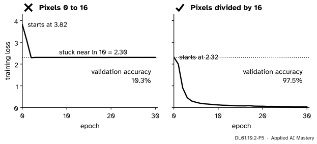
DL01.10.2-F5
Wrong beside right. With unscaled pixels the first steps are so large that every hidden unit dies, and the network can only learn the class shares: the loss of a constant guess, about \(\ln 10\).
“I forgot to divide by 16, but the network will adapt.”
With pixel values up to 16 the pre-activations are up to 16 times larger, the starting loss is 3.82 instead of 2.32 (check 1 fails at once), and the first updates with learning rate 0.3 push every one of the 32 hidden units below zero on every training image. A dead ReLU passes no gradient (DL01.3.2), so the output becomes a constant and validation accuracy sits at the majority baseline’s 10.3 percent.
“Width 64 scored 352 and width 32 scored 351, so 64 is better.”
One image in 360 is far less than one standard error (2.8 images). Another validation set could reverse the order. The rule keeps the smaller network unless the bigger one is clearly better.
“Pick the run with the lowest training loss.”
The widest network with the largest learning rate nearly always wins that contest, because it can memorise more. Training loss measures fitting, not generalising (ML01.8); every choice here is made on validation.
“The checks are a waste of time; just train.”
Each takes a second. A loop with a bug often still produces a falling loss, but rarely the right starting value and a batch driven to zero (DL01.8.3).
Check yourself
Recall
1. How many parameters does the 64-32-10 network have, layer by layer?
Show answer
\({32 \cdot 65 = 2{,}080}\) in the first layer and \({10 \cdot 33 = 330}\) in the second: 2,410.
2. Why should the loss of a fresh ten-class network start near 2.303?
Show answer
Its logits are nearly equal, and with equal logits \({-z_y + \ln \sum_k e^{z_k} = \ln 10 \approx 2.303}\).
3. What does the one-batch check test, and what result do we want?
Show answer
That the loop can fit at all: training repeatedly on 32 images should drive their loss close to zero (here 0.02 after 200 steps).
4. State the one-standard-error rule.
Show answer
Among runs whose validation count is within one standard error of the best, keep the one with the fewest parameters, and between equal sizes the higher count.
5. Which run did the grid keep, and with what validation score?
Show answer
Width 32 and learning rate 0.3, epoch 21: 351 of 360, 97.5 percent.
Exercises
1.★ Count the parameters of the 64-16-10 and 64-64-10 networks, and the updates in a run of 50 epochs with batches of 64 on the 1,077 training images.
With batches of 64 an epoch has \({\lceil 1077/64 \rceil = 17}\) steps (16 full batches and one of 53), so 50 epochs make \({50 \cdot 17 = 850}\) updates.
2.★★ Another grid gives validation counts, out of 360, of 340 for width 16, 346 for width 32 and 347 for width 64. Apply the one-standard-error rule.
Show solution
The best is 347: \({p^* = 0.9639}\), \({p^*(1 - p^*) = 0.0348}\), divided by 360 is \({9.67 \times 10^{-5}}\), square root 0.00983, so \({s = 360 \cdot 0.00983 = 3.54}\) images. The floor is \({347 - 3.54 = 343.5}\): widths 32 (346) and 64 (347) are inside, width 16 (340) is not. Keep width 32.
3.★★★ A network whose hidden units are all dead outputs the same logits for every image. Show that the lowest mean cross-entropy it can reach on the training set is the entropy of the class shares, \({H = -\sum_k q_k \ln q_k}\) with \({q_k = n_k / n}\), and compute it for the training counts (107, 109, 106, 109, 109, 109, 109, 107, 104, 108).
Show solution
A constant output gives the same probabilities \(p_k\) to every image, so the mean loss is \({-\frac{1}{n}\sum_i \ln p_{y_i} = -\sum_k q_k \ln p_k}\), because \(n_k\) images have label \(k\). Write this as \({H + \sum_k q_k \ln (q_k / p_k)}\). The second term is the Kullback-Leibler divergence of DL01.4.3, and it is never negative. To see why, use \({\ln u \le u - 1}\), with equality only at \({u = 1}\):
with equality only when every \({p_k = q_k}\). So the minimum is \(H\), reached by predicting the class shares. For these counts \({H = 2.3025}\), a hair below \({\ln 10 = 2.3026}\) because the shares are nearly equal. The unscaled run of the pitfall ends at 2.306, close to this floor.
Summary card
Check the loop, train with fit, choose on validation with the one-standard-error rule.
DL01.10.2-F1
From \(\ln 10\) to 97.5 percent in 21 epochs.
Parameters: \({n_{\text{out}}(n_{\text{in}} + 1)}\) per layer; 64-32-10 has 2,410.
Check 1: starting loss near \({\ln 10 = 2.303}\). Check 2: one batch driven to nearly zero.
Standard error of a count: \({s = n\sqrt{p^*(1-p^*)/n}}\), here 2.8 images.
Kept: width 32, learning rate 0.3, epoch 21, 351 of 360 on validation.
Sources and next steps
Sources. Each was opened and checked against this lesson on 15 November 2026.
PyTorch 2.15 documentation, torch.nn.Linear: the weight has shape (out_features, in_features) and, like the bias, starts uniform on \({(-\sqrt{k}, \sqrt{k})}\) with k = 1/in_features, which is why the first logits are small.
PyTorch 2.15 documentation, torch.nn.CrossEntropyLoss: the input holds unnormalised logits, the target holds class indices, and the default reduction is the mean.
PyTorch 2.15 documentation, torch.optim.SGD: the signature and its defaults (lr=0.001, no momentum, no weight decay); this lesson passes lr itself.
scikit-learn 1.9 examples, Balance model complexity and cross-validated score: states the one-standard-error rule, select the simplest model whose performance is within one standard error of the best, citing Hastie, Tibshirani and Friedman, The Elements of Statistical Learning, the chapter on model assessment and selection.