Open the test set for the one and only time: report the network’s accuracy with a binomial standard error, compare it with logistic regression image by image, and read the confusion matrix, the most confused pairs and the misclassified images.
DL01.10.3L2 Intermediate25 minIn review (what this means)
The maths and code on this page are checked by automated tests on every change, but an independent reader has not signed it off yet. Spot a mistake or a confusing step? Tell us.
Evaluate the chosen network once on the test set and explain why its score is lower than the validation score.
Derive the binomial standard error of an accuracy from the standard error of a mean, and attach it to a reported accuracy.
Compare two classifiers on the same test images with the paired standard error of their gap.
Read a confusion matrix: recall and precision of a class, and the most confused pairs.
The question
The network got 97.5 percent of the validation images right and was chosen for it. What will it score on images that played no part in any decision, how sure can we be of that number, and is it really better than the logistic regression it was meant to beat?
From the last lesson
1. Which run did the grid keep, and why not the run with the highest validation count?
Show answer
Width 32 and learning rate 0.3 (351 of 360). Width 64 scored 352, but one image is well inside one standard error (2.8 images), so the one-standard-error rule keeps the smaller network.
2. What does a starting loss far above \(\ln 10\) tell you?
Show answer
The logits are already large and confidently wrong before training: something such as unscaled inputs is off, and the loop should not be trusted yet.
Intuition
The test set has been closed since the split. Now it is opened once, for one measurement, and nothing is changed afterwards. That single number is the honest estimate of how the network will do on new digits. Then we look inside it: which digits are mistaken for which.
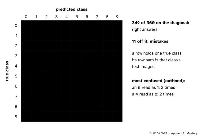
DL01.10.3-F1
The confusion matrix of the chosen network on the 360 test images. Right answers lie on the diagonal; every mistake is a cell off it, in the row of the true class and the column of the answer.
The picture says three things at once. Most of the weight is on the diagonal. The mistakes are scattered, never more than two in a cell. And they make sense to a human eye: an 8 read as a 1, a 4 read as an 8, a 9 read as a 5. A mistake that looks like a plausible confusion is reassuring; a whole row of mistakes would point at a bug.
Build it up
Step 1. Rebuild the chosen network. Training is seeded, so running the training of DL01.10.2 again with width 32 and learning rate 0.3 gives the same weights, and 351 validation images right.
Step 2. Test once. It gets 349 of the 360 test images right: 96.9 percent. That is lower than its 97.5 percent on validation, and it should be. The validation score was the best of nine runs and thirty epochs, so it carries a little luck that the choice selected for; the test score carries none (ML01.9.4).
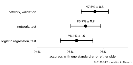
Step 3. Attach an error bar. A different set of 360 test images would give a slightly different count. The binomial standard error, derived below, is 0.9 percentage points here: the test accuracy is \({96.9 \pm 0.9}\) percent.
DL01.10.3-F2
Each accuracy with one standard error either side. The validation score (hollow) is the one that was used for choosing, so it is the least trustworthy of the three.
Step 4. The baseline on the same images. Logistic regression gets 347 of 360: 96.4 percent. The network is two images ahead. Is that a real lead? The formal statement answers with a second standard error, for the gap.
Step 5. Read the matrix. Row \(k\) holds the test images whose true class is \(k\); column \(j\) holds those the network called \(j\). The recall of class \(k\) is its diagonal cell divided by its row sum; its precision is the diagonal cell divided by its column sum. Class 8 has the lowest recall, 32 of 35, and class 1 the lowest precision: 39 images were called 1, and only 35 of them were ones.
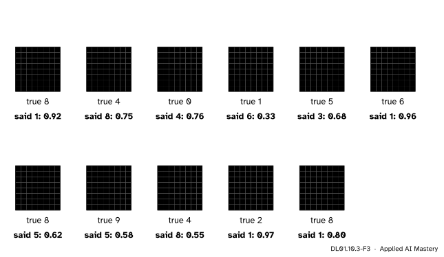
Step 6. Look at the mistakes. Numbers say how often; pictures say why.
DL01.10.3-F3
All eleven test images the network gets wrong. Several are hard for a person too; three of the wrong answers come with a probability above 0.9.
The formal statement
NoteThe standard error of an accuracy
Let \({c_j = 1}\) if test image \(j\) is classified correctly and 0 if not, for \({j = 1, \dots, n}\), and let \({\hat{p} = \tfrac{1}{n}\sum_j c_j}\) be the accuracy. Then its standard error is
Derivation. The accuracy is the mean of the \(n\) numbers \(c_j\), and ML01.2.3 gives the standard error of a mean of per-example values as \({s/\sqrt{n}}\), where \(s\) is their standard deviation. Because each \(c_j\) is 0 or 1, \({c_j^2 = c_j}\), so the mean of the squares is \(\hat{p}\) too, and
Dividing \(s\) by \(\sqrt{n}\) gives the formula. (With the divisor \({n - 1}\) in \(s^2\) the result grows by the factor \({\sqrt{n/(n-1)}}\), which is 1.0014 for 360 images.) The count of right answers is binomial, which gives the formula its name.
NoteThe standard error of a gap, on the same images
Let \({d_j = c_j^{\text{net}} - c_j^{\text{base}}}\). Let \(b\) count the images only the network gets right and \(c\) those only the baseline gets right. The gap in accuracy is \({\bar{d} = (b - c)/n}\) and
Derivation. Each \(d_j\) is \(+1\) on the \(b\) images only the network gets right, \(-1\) on the \(c\) images only the baseline gets right, and 0 where they agree. So \({\sum_j d_j = b - c}\), and \({d_j^2 = 1}\) exactly on the \({b + c}\) images where they disagree. The same steps as above give
and dividing \(s_d\) by \(\sqrt{n}\) gives the formula. Only the images where the two models disagree carry information about which is better. Treating the two accuracies as independent would give \({\sqrt{\text{SE}_1^2 + \text{SE}_2^2}}\), about twice as large here, because it ignores that both models get the same 345 images right.
Worked example
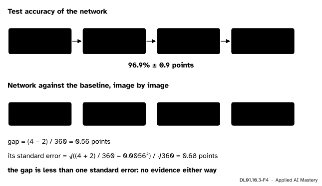
The network’s test accuracy. It is right on 349 of 360 images, so \({\hat{p} = 0.9694}\). Then \({\hat{p}(1 - \hat{p}) = 0.9694 \cdot 0.0306 = 0.0296}\), divided by 360 is \({8.23 \times 10^{-5}}\), and the square root is 0.0091. Report: 96.9 percent, standard error 0.9 points.
The gap to the baseline. Image by image, both are right on 345, only the network on \({b = 4}\), only the baseline on \({c = 2}\), and both wrong on 9. The gap is \({\bar{d} = (4 - 2)/360 = 0.0056}\), 0.56 points. Its standard error:
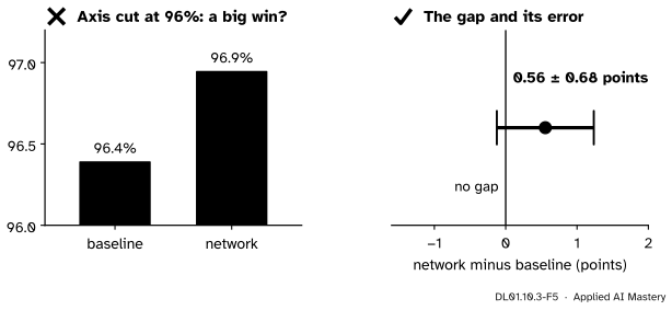
The gap, 0.56 points, is smaller than one standard error, 0.68 points. On this test set the network is not shown to be better than logistic regression. Six images out of 360 separate the two models, and they split four to two.
DL01.10.3-F4
The two standard errors of this lesson, computed step by step.
Code
The data, and the training of DL01.10.2 condensed into one function that keeps the epoch with the lowest validation loss.
validation images right: 351 of 360 (as in DL01.10.2)
The one test of the project, with its standard error, and the baseline on the same images.
with torch.no_grad(): probs = model(t(X_test)).softmax(dim=1).numpy()pred = probs.argmax(axis=1)right_net = pred == y_testbase = LogisticRegression(max_iter=1000).fit(X_train, y_train)right_base = base.predict(X_test) == y_testdef se(p, n=360):return math.sqrt(p * (1- p) / n)p_net, p_base = right_net.mean(), right_base.mean()print(f"network: {right_net.sum()} of 360 = {p_net:.4f}, standard error {se(p_net):.4f}")print(f"baseline: {right_base.sum()} of 360 = {p_base:.4f}, standard error {se(p_base):.4f}")d = right_net.astype(float) - right_base.astype(float)b, c =int((d ==1).sum()), int((d ==-1).sum())gap = d.mean()se_gap = math.sqrt(((b + c) /360- gap **2) /360)print(f"only the network right: {b}, only the baseline right: {c}, both right: {(right_net & right_base).sum()}")print(f"gap {gap:.4f}, paired standard error {se_gap:.4f} (np.std gives {d.std() / math.sqrt(360):.4f}); "f"as if independent {math.sqrt(se(p_net) **2+ se(p_base) **2):.4f}")
network:  349 of 360 = 0.9694, standard error 0.0091
baseline: 347 of 360 = 0.9639, standard error 0.0098
only the network right: 4, only the baseline right: 2, both right: 345
gap 0.0056, paired standard error 0.0068 (np.std gives 0.0068); as if independent 0.0134
The paired formula and np.std of the differences agree, as derived. Ignoring the pairing doubles the error bar.
The confusion matrix, the most confused pairs and the report. Rows are true classes, columns predictions, as the scikit-learn documentation defines them.
cm = confusion_matrix(y_test, pred)print(cm)pairs =sorted(((cm[i, j], i, j) for i inrange(10) for j inrange(10) if i != j and cm[i, j]), reverse=True)print("most confused (count, true, predicted):", [tuple(int(v) for v in p) for p in pairs[:3]])print("recall of class 8:", round(cm[8, 8] / cm[8].sum(), 3), " precision of class 1:", round(cm[1, 1] / cm[:, 1].sum(), 3))print(classification_report(y_test, pred, digits=3))
Finally the mistakes themselves, with the network’s confidence in each wrong answer.
wrong = np.flatnonzero(~right_net)for j in wrong:print(f"image {j:3d}: true {y_test[j]}, said {pred[j]} with p = {probs[j, pred[j]]:.2f}, "f"p(true) = {probs[j, y_test[j]]:.2f}")print("confident mistakes (p > 0.9):", int((probs[wrong, pred[wrong]] >0.9).sum()))
image  15: true 8, said 1 with p = 0.92, p(true) = 0.06
image  56: true 4, said 8 with p = 0.75, p(true) = 0.00
image  70: true 0, said 4 with p = 0.76, p(true) = 0.24
image 179: true 1, said 6 with p = 0.33, p(true) = 0.02
image 207: true 5, said 3 with p = 0.68, p(true) = 0.20
image 209: true 6, said 1 with p = 0.96, p(true) = 0.02
image 219: true 8, said 5 with p = 0.62, p(true) = 0.30
image 240: true 9, said 5 with p = 0.58, p(true) = 0.07
image 242: true 4, said 8 with p = 0.55, p(true) = 0.00
image 291: true 2, said 1 with p = 0.97, p(true) = 0.01
image 333: true 8, said 1 with p = 0.80, p(true) = 0.17
confident mistakes (p > 0.9): 3
Explore
The digit sketchpad of DL01.10.4 runs this network. Its Next test image button reaches three of the mistakes above, an 8 read as a 1, a 1 read as a 6 and a 4 read as an 8. Paint over one of them a cell at a time and watch how few strokes it takes to tip the answer back.
Pitfalls
DL01.10.3-F5
Wrong beside right. Cutting the axis turns half a point into a towering lead. The gap with its own standard error shows that zero is well within reach.
“The test score is lower than the validation score, so something went wrong.”
It is expected. The validation score was the best of many and was used to choose; the test score was used for nothing. A test score far below validation, by many standard errors, would deserve a look; 0.6 points is not that.
“Test accuracy is a bit disappointing; let me try width 64 and test again.”
Then the test set has become a second validation set, and the new number is optimistic in the same way (ML01.9.4). Any change after the test means a new, untouched test set for an honest number.
“96.9 against 96.4: the network beats logistic regression.”
The gap is 2 images in 360, smaller than its standard error. What the test shows is that both are about 96 to 97 percent accurate on these digits. Lesson DL01.10.4 shows a reason: on 8 by 8 images a hidden layer has little that a linear model cannot already reach.
“The cell in row 1, column 8 counts eights called ones.”
In scikit-learn’s convention the row is the truth and the column the prediction, so that cell counts ones called eights. Check the convention of any matrix before reading it; some books transpose it.
Check yourself
Recall
1. What is the network’s test accuracy, with its standard error?
Show answer
349 of 360, 96.9 percent, with a standard error of 0.9 points.
2. Why is \({s^2 = \hat{p}(1 - \hat{p})}\) for the right-or-wrong values \(c_j\)?
Show answer
Because \({c_j^2 = c_j}\) for values 0 and 1, so the mean of the squares is \(\hat{p}\) and \({s^2 = \hat{p} - \hat{p}^2}\).
3. Which images carry information about which of two classifiers is better?
Show answer
Only those where they disagree; the paired standard error depends on the counts \(b\) and \(c\) alone.
4. How do you read the recall and the precision of class \(k\) off a confusion matrix?
Show answer
Recall: the diagonal cell over its row sum. Precision: the diagonal cell over its column sum.
5. Which classes does the network confuse most often on the test set?
Show answer
Eights called ones and fours called eights, twice each.
Exercises
1.★ A model gets 340 of 360 test images right. Give its accuracy with its standard error, and say how many test images you would need to halve that error.
Show solution
\({\hat{p} = 340/360 = 0.9444}\), \({\hat{p}(1 - \hat{p}) = 0.0525}\), divided by 360 is \({1.46 \times 10^{-4}}\), square root 0.0121: 94.4 percent, standard error 1.2 points. The error falls as \({1/\sqrt{n}}\), so halving it needs four times the images, 1,440.
2.★★ From the confusion matrix of this lesson, compute the recall and the precision of class 8. Column 8 holds 32 on the diagonal and 2 from row 4.
Show solution
Row 8 holds 35 test images, of which 32 are on the diagonal: recall \({32/35 = 0.914}\). Column 8 holds \({32 + 2 = 34}\) images called 8, of which 32 are eights: precision \({32/34 = 0.941}\). Both match the classification_report.
3.★★★ Two classifiers are tested on the same 360 images. Each gets 340 right. Find the paired standard error of their gap when they disagree on no image, and when each is right on 10 images the other gets wrong. What does the comparison teach about pairing?
Show solution
In both cases the gap is 0. With no disagreements \({b = c = 0}\) and the standard error is 0: the two make exactly the same predictions, so there is nothing to distinguish them. With \({b = c = 10}\),
that is 1.2 points. The two accuracies and their own standard errors (1.2 points each) are the same in both cases; only the pattern of agreement changes the error of the gap. That is why two models must be compared on the same images, image by image.
Summary card
Test once, with an error bar, and read the mistakes.
DL01.10.3-F1
349 right, 11 mistakes, none in bulk.
Test accuracy: 349 of 360, \({96.9 \pm 0.9}\) percent; the baseline \({96.4 \pm 1.0}\).
\({\text{SE}(\hat{p}) = \sqrt{\hat{p}(1 - \hat{p})/n}}\), from \({c_j^2 = c_j}\).
Row = truth, column = answer; recall by rows, precision by columns.
Sources and next steps
Sources. Each was opened and checked against this lesson on 15 November 2026.
scikit-learn 1.9 API reference, confusion_matrix: entry \({(i, j)}\) is the number of observations known to be in group \(i\) and predicted to be in group \(j\), so rows are true classes and columns predictions.
scikit-learn 1.9 API reference, classification_report: precision, recall, F1 and support per class, with the macro and the support-weighted averages.
scikit-learn 1.9 user guide, Toy datasets: the UCI digits were written by 43 people, 30 for its training part and 13 others for its test part, and load_digits is a copy of that test part; the 8 by 8 values count on pixels in 4 by 4 blocks, which blurs strokes and is part of why some mistakes above are hard even for a person.