Swap two hidden units, or flip the signs of a tanh unit’s weights, and the network computes the same function from different weights. So every minimum has copies, and the loss of a network cannot be convex. Slices along a line and over a plane make the surface visible.
DL01.4.4L2 Intermediate25 minIn review (what this means)
The maths and code on this page are checked by automated tests on every change, but an independent reader has not signed it off yet. Spot a mistake or a confusing step? Tell us.
Show that permuting hidden units, and flipping the signs of a tanh unit’s weights in and out, leave a network’s function unchanged, and count the H! 2^H copies for H tanh hidden units.
Use two equal-loss copies of a network to prove that its loss is not a convex function of the weights.
Compute the loss along the straight line between two weight vectors, and over a plane through the trained weights along two random directions.
Explain why averaging the weights of two trained networks needs their hidden units aligned first.
The question
The loss of linear regression is a bowl with one bottom (ML01.5.1), so gradient descent cannot go wrong for long. The loss of a network depends on all its weights at once: nine numbers for the small XOR network of M05.9, millions for a real one. Is that surface still a bowl? If not, what shape is it, and how can anyone look at a surface in nine or a million dimensions?
From the last lesson
1. Write categorical cross-entropy for logits \(\vect{z}\) and true class \(k\).
Show answer
\({\ell = -z_k + \mathrm{LSE}(\vect{z})}\), with \({\mathrm{LSE}(\vect{z}) = \ln\sum_j e^{z_j}}\).
2. Why does subtracting the largest logit keep the computation safe, and why is the answer unchanged?
Show answer
Every exponent becomes at most 0, so nothing overflows. The softmax is unchanged when the same constant is added to every logit, because the factor \(e^{c}\) cancels.
Intuition
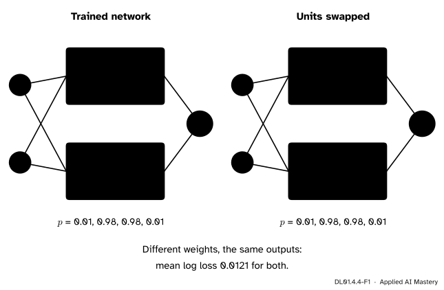
Take the XOR network of M05.9: two inputs, two tanh hidden units, one sigmoid output, trained with the mean log loss. Call its hidden units A and B. Nothing in the network says which unit is “first”. Swap them, moving each unit’s incoming weights, bias and outgoing weight together, and the output is the sum of the same two contributions in the other order.
DL01.4.4-F1
The trained XOR network and the same network with its hidden units swapped. The weight vectors differ, the outputs on the four XOR points do not, and neither does the loss.
So the same function sits at two different points of weight space, and so does its loss. A bowl has one bottom; a surface with two equally low points cannot be a bowl. Between them, as we shall see, the loss climbs.
Build it up
Step 1. The trained network. Start from the weights fixed in M05.9.1 and take 300 full-batch gradient-descent steps with learning rate 1, as in M05.9.2. The mean log loss falls from 0.872 to 0.0121. Call the result \(\theta^*\): nine numbers, rounded to one decimal in the figure.
Step 2. Swapping. With \({u_A}\) and \({u_B}\) the pre-activations of the two hidden units, the output logit is
Exchanging everything that belongs to A with everything that belongs to B only reorders a sum. With \(H\) hidden units there are \({H!}\) orders, so \({H!}\) weight vectors per function.
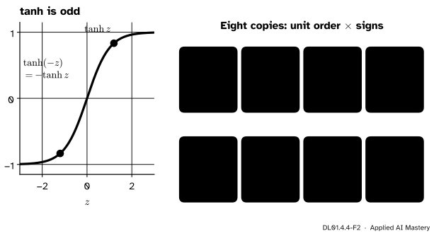
Step 3. Flipping signs. The tanh is an odd function: \({\tanh(-u) = -\tanh u}\). Multiply a unit’s incoming weights and bias by \(-1\); its pre-activation changes sign, so its output changes sign. Multiply its outgoing weight by \(-1\) too, and its contribution to \(z\) is back to what it was:
Each of the \(H\) units can be flipped or not, independently: \({2^H}\) choices.
DL01.4.4-F2
Left: tanh is odd, so a sign flip in and out cancels. Right: two orders times four sign patterns give eight weight vectors with the same loss, 0.0121.
Step 4. Count them. Orders and signs combine freely, so in a network with \(H\) tanh hidden units in one layer every weight vector has
\[
H! \times 2^H
\]
copies that compute the same function, itself included. They are all different unless two units have equal or opposite weights, or a unit’s weights are all 0. For the XOR network, \({2! \times 2^2 = 8}\), all different. For one layer of 100 tanh units the count is \({100! \times 2^{100}}\), a number with 189 digits. Every point of weight space, and in particular every minimum, comes with all its copies.
The formal statement
NoteConvexity, and why a network’s loss lacks it
A loss \(L\) is convex if for any two weight vectors \(\theta\) and \(\theta'\) and every \({\alpha \in [0, 1]}\),
The mean log loss of the XOR network is not convex.
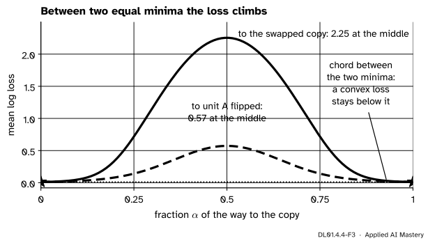
Proof. Let \(\theta'\) be \(\theta^*\) with its hidden units swapped, so \({L(\theta') = L(\theta^*) = 0.0121}\). If \(L\) were convex, the right-hand side would be \({(1-\alpha)\,0.0121 + \alpha\,0.0121 = 0.0121}\) for every \(\alpha\), so the loss could nowhere on the segment rise above 0.0121. At the midpoint \({\alpha = \tfrac12}\) the two hidden units become identical, with incoming weights \({(3.30, -3.27)}\) and bias \({-0.09}\), and their outgoing weights, 5.01 and \({-5.04}\), average to about \({-0.02}\) each. The hidden layer is all but switched off, the output bias of 4.48 alone sets every prediction to about 0.99, and the loss is 2.254. That breaks the inequality, so \(L\) is not convex. ∎
DL01.4.4-F3
The loss along the straight line from \(\theta^*\) to two of its copies. Both ends are equally low, and in between the loss climbs far above the chord: 2.25 towards the swapped copy and 0.57 towards the copy with unit A flipped.
The argument uses nothing special about XOR. Any network with two or more interchangeable hidden units has copies, and the straight line between two copies generally passes through networks that compute something else. Convex losses, like those of linear and logistic regression, have the property that every local minimum is a global one; a network’s loss gives up that guarantee.
Go deeper: other symmetries, and why this one is harmless
ReLU units have a symmetry of their own: multiply a unit’s incoming weights and bias by any \({c > 0}\) and divide its outgoing weight by \(c\), and \({\mathrm{relu}(cu)/c = \mathrm{relu}(u)}\) leaves the function unchanged (Prince, Section 20.3.1). That gives a whole curve of equivalent weights through every point. These symmetries do not make training harder by themselves: the copies are equally good, so it does not matter which one gradient descent finds. What they do show is that “the” minimum of a network is never one point, and that pictures of the surface must be read with care.
Worked example
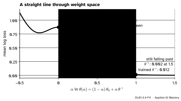
A surface over nine numbers cannot be drawn, but a line through it can. Goodfellow, Vinyals and Saxe (2015) evaluate the loss along the straight line from the starting weights \(\theta_0\) to the trained weights \(\theta^*\):
The loss along the straight line from the start to the trained weights falls without a single bump. Past \({\alpha = 1}\) it keeps falling: on XOR the loss has no lowest point at finite weights.
Read three things from it. The loss falls all the way from start to finish, with no wall to climb: this is what Goodfellow and colleagues found for much larger networks too. The path gradient descent actually took was not this straight line, so the picture says the start and the end are connected by an easy road, not that training used it. And beyond \({\alpha = 1}\) the loss keeps falling, to 0.002 at \({\alpha = 1.5}\): the four XOR points can be separated, so making the weights larger keeps sharpening the probabilities towards 0 and 1, and the loss approaches 0 without reaching it. “The trained weights” are where we stopped, not a bottom.
Code
The network and its training, written as in M05.9.2 with the nine parameters in one vector, so that weight vectors can be added and scaled.
import itertoolsimport numpy as npX = np.array([[0.0, 0.0], [0.0, 1.0], [1.0, 0.0], [1.0, 1.0]])y = np.array([0.0, 1.0, 1.0, 0.0])def unpack(th):return th[:4].reshape(2, 2), th[4:6], th[6:8], th[8]def loss(th): W1, b1, w2, b2 = unpack(th) z = np.tanh(X @ W1.T + b1) @ w2 + b2return np.mean(np.logaddexp(0.0, z) - y * z) # softplus(z) - y z, as in DL01.4.2def grad(th): W1, b1, w2, b2 = unpack(th) A = np.tanh(X @ W1.T + b1) d2 = (1/ (1+ np.exp(-(A @ w2 + b2))) - y) /len(y) # p - y, over n D1 = np.outer(d2, w2) * (1- A **2)return np.concatenate([(D1.T @ X).ravel(), D1.sum(0), A.T @ d2, [d2.sum()]])def train(th, steps=300, lr=1.0):for _ inrange(steps): th = th - lr * grad(th)return thstart = np.array([1.0, -1.0, 0.5, 0.5, 0.0, 0.0, 2.0, -1.0, 0.0]) # M05.9.1best = train(start)print(f"loss at the start {loss(start):.3f}, after 300 steps {loss(best):.4f}")def relabel(th, order, signs): W1, b1, w2, b2 = unpack(th) o, s =list(order), np.array(signs, dtype=float)return np.concatenate([(s[:, None] * W1[o]).ravel(), s * b1[o], s * w2[o], [b2]])copies = [relabel(best, o, s) for o in itertools.permutations([0, 1]) for s in itertools.product([1, -1], repeat=2)]losses = [loss(c) for c in copies]print(f"eight copies: losses from {min(losses):.6f} to {max(losses):.6f},","distinct vectors:", len({tuple(np.round(c, 6)) for c in copies}))swap = relabel(best, [1, 0], [1, 1])print(f"loss at the midpoint between theta* and its swapped copy: {loss((best + swap) /2):.3f}")
loss at the start 0.872, after 300 steps 0.0121
eight copies: losses from 0.012058 to 0.012058, distinct vectors: 8
loss at the midpoint between theta* and its swapped copy: 2.254
Now the two slices: the straight line from start to finish, and a plane through \(\theta^*\) spanned by two random directions of length 1, the second made perpendicular to the first.
alphas = np.linspace(0, 1, 101)line = np.array([loss((1- a) * start + a * best) for a in alphas])print("along the line at 0, 0.25, 0.5, 0.75, 1:", line[::25].round(3))print("falls at every step:", bool(np.all(np.diff(line) <0)), " at alpha = 1.5:", round(loss(-0.5* start +1.5* best), 4))rng = np.random.default_rng(0)d1, d2 = rng.normal(size=(2, 9))d1 /= np.linalg.norm(d1)d2 -= (d2 @ d1) * d1d2 /= np.linalg.norm(d2)steps = np.linspace(-6, 6, 61)plane = np.array([[loss(best + a * d1 + b * d2) for a in steps] for b in steps])print(f"on the plane: lowest {plane.min():.4f} at the centre: {plane.argmin() == plane.size //2},"f" highest {plane.max():.2f}")
along the line at 0, 0.25, 0.5, 0.75, 1: [0.872 0.617 0.209 0.046 0.012]
falls at every step: True   at alpha = 1.5: 0.0015
on the plane: lowest 0.0121 at the centre: True, highest 6.23
The random directions come from a seeded generator; a different seed gives a different plane, and a different picture of the same surface.
Explore
There is no interactive for this lesson; the module’s one-example loss explorer is in lesson DL01.4.2. Here is the plane the code computed.
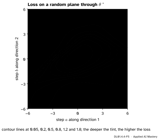
DL01.4.4-F5
The loss on a plane through \(\theta^*\) along two random unit directions. Near \(\theta^*\) it looks like a lopsided bowl; further out the contours twist. One plane shows two of nine dimensions.
Things to notice. The lowest point of this plane is \(\theta^*\) itself, though the line slice showed that the loss keeps falling in another direction: a plane only sees the directions it contains. And the copies of \(\theta^*\) are nowhere in the picture, because a random plane almost never passes through them. Li and colleagues (2018) used exactly such planes, with an extra rescaling of the directions called filter normalisation that DL10.2 explains.
Pitfalls
DL01.4.4-F6
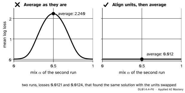
Wrong beside right. A second run from random starting weights finds the same solution with its hidden units in the other order. Averaging the two as they are gives a loss of 2.240; putting the second network’s units in the first one’s order first gives 0.012.
“Two trained networks are both good, so their average is good too.”
Only if their hidden units correspond. Training from a different start can find the same solution with the units permuted, or with signs flipped, and the average of two such networks sits on the bump between copies. Aligning first, by choosing the copy of the second network nearest the first, fixes it in this example. The same care is needed whenever weights are averaged.
“The loss along the line from start to finish shows the path training took.”
It shows a straight road between two points. Gradient descent took a curved path, step by step, and may have passed through regions this line never visits. The slice is evidence about the surface, not a record of the run.
“A two-dimensional slice shows the shape of the loss surface.”
It shows two directions out of nine here, and out of millions in a real network. The same surface looks different on a different plane, and features such as the copies of a minimum can be invisible on all the planes one happens to draw.
Check yourself
Recall
1. Name two changes to a tanh network’s weights that leave its function unchanged.
Show answer
Permuting the hidden units, moving each unit’s incoming weights, bias and outgoing weight together; and multiplying a unit’s incoming weights, bias and outgoing weight by \(-1\).
2. How many copies do these changes make of a weight vector of a network with one layer of \(H\) tanh hidden units, and how many for the XOR network?
Show answer
\({H! \times 2^H}\); for \({H = 2}\) that is \({2 \times 4 = 8}\).
3. How do two copies of the same network prove that its loss is not convex?
Show answer
They have equal loss, so a convex loss could not rise above that value anywhere on the segment between them. At the midpoint it does: 2.254 against 0.0121 for the XOR network.
4. What does the slice \({L((1-\alpha)\theta_0 + \alpha\theta^*)}\) show, and what does it not show?
Show answer
The loss along the straight line from the start to the trained weights: for the XOR network it falls all the way. It does not show the path that gradient descent actually took.
5. Why does the XOR loss keep falling past the trained weights?
Show answer
The four points can be separated, so scaling the weights up sharpens every probability towards the right label. The loss approaches 0 but has no lowest point at finite weights.
Exercises
1.★ A network has one hidden layer of 3 tanh units. How many copies of a weight vector do permutations and sign flips give? How many with two hidden layers of 3 tanh units each?
Show solution
One layer: \({3! \times 2^3 = 6 \times 8 = 48}\). Each hidden layer has its own orders and signs, independently, so two layers give \({48 \times 48 = 2{,}304}\).
2.★★ Flip the signs of unit A’s weights in and out and take the midpoint between \(\theta^*\) and that copy. What are unit A’s incoming weights, bias and outgoing weight there, and what does unit A contribute to the output?
Show solution
Each of unit A’s weights is averaged with its own negative, so all of them are 0. Its output is \({\tanh(0) = 0}\), multiplied by an outgoing weight of 0: it contributes nothing. The network is reduced to unit B alone, which cannot solve XOR, and the loss is 0.573 (figure DL01.4.4-F3).
3.★★★ Show that if \(L\) is convex and \({L(\theta) = L(\theta') = c}\), then \({L \le c}\) everywhere on the segment between them, and that a convex \(L\) whose lowest value \(c\) is reached at two points is also lowest at every point between them. Why can’t the XOR loss be “convex with a flat valley” between \(\theta^*\) and its copies?
Show solution
Convexity gives \({L((1-\alpha)\theta + \alpha\theta')} \le {(1-\alpha)c + \alpha c} = c\). If \(c\) is the lowest value, \(L\) is also at least \(c\) everywhere, so \({L = c}\) on the whole segment: a flat valley. For XOR, the loss at the midpoint between \(\theta^*\) and its swapped copy is 2.254, far above 0.0121, so no flat valley joins them, and \(L\) cannot be convex.
Summary card
Equal copies of every network make the loss surface many-valleyed.
DL01.4.4-F1
Swap the units: same function, new weights.
Symmetries: permute hidden units; flip a tanh unit’s signs in and out. \({H! \times 2^H}\) copies.
Not convex: two copies have equal loss, the midpoint between them a higher one (2.254 for XOR).
Line slice:\({L((1-\alpha)\theta_0 + \alpha\theta^*)}\), from start to trained weights.
Plane slice:\({L(\theta^* + a\,\vect{d}_1 + b\,\vect{d}_2)}\), two random unit directions.
Sources and next steps
Sources. Each was opened and checked against this lesson on 15 November 2026.
Christopher M. Bishop, Pattern Recognition and Machine Learning, Springer, 2006 (free PDF from Microsoft Research). Section 5.1.1, weight-space symmetries: the sign flip of a tanh unit, the interchange of hidden units, and the factor \({M!\,2^M}\) for \(M\) hidden units.
Ian J. Goodfellow, Oriol Vinyals and Andrew M. Saxe, Qualitatively characterizing neural network optimization problems, ICLR 2015. Section 2 evaluates the objective at \({\theta = (1-\alpha)\theta_0 + \alpha\theta_1}\) and reports that from the initial to the final parameters it is simple and approximately convex.
Hao Li, Zheng Xu, Gavin Taylor, Christoph Studer and Tom Goldstein, Visualizing the Loss Landscape of Neural Nets, NeurIPS 2018. Section 3 describes the one-dimensional interpolation and the plots \({f(\alpha, \beta) = L(\theta^* + \alpha\delta + \beta\eta)}\) along two random directions (equation 1); Section 4 introduces filter normalisation.
Simon J. D. Prince, Understanding Deep Learning, MIT Press, 2023 (free PDF). Section 20.3.1 on the many equivalent global minima from permuting hidden units and rescaling around ReLUs; Sections 20.3.2 and 20.3.3 on straight lines from the start to the minimum and between minima.
Next. DL01.5 Backpropagation by hand computes, number by number, the gradients that move a network across this surface.