Fix the course’s split of the digits once: stratified twice into 1,077 training, 360 validation and 360 test images. See why random_split does not stratify, then let samplers and class weights rescue a class cut to a tenth of its images.
DL01.9.4L2 Intermediate30 minIn review (what this means)
The maths and code on this page are checked by automated tests on every change, but an independent reader has not signed it off yet. Spot a mistake or a confusing step? Tell us.
Split load_digits into 1,077 training, 360 validation and 360 test images with two stratified calls to train_test_split, and explain the rounding.
Use random_split and Subset, and explain why random_split does not keep the class mix.
Show that a WeightedRandomSampler with weights 1/n_k draws each class with probability 1/K, and that class weights n/(K n_k) give each class the same total weight in the loss.
Compare the sampler and the class weights on a training set with one class cut to a tenth, by per-class recall.
The question
Split 1,797 digit images at random and one class can end up with 27 validation images while another gets 43. Worse, if one class is rare in the training data, a network can learn to never predict it and still score 86 percent. How do you split so that every part keeps the class mix, and how do you make training pay attention to a rare class?
From the last lesson
1. What is the spread of a batch gradient of \(\abs{B}\) independent draws, in terms of the gradient variance \(\sigma^2\)?
Show answer
\(\sigma^2 / \abs{B}\); drawn without replacement, times \({(n - \abs{B})/(n - 1)}\).
2. On 1,077 images, how many updates does one epoch give with batches of 8, and with batches of 512?
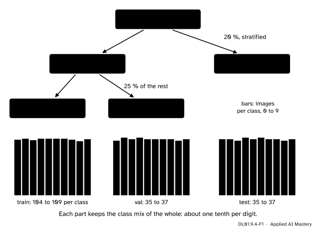
A stratified split cuts each class separately in the same proportions, then puts the pieces together. Every part then holds about the same share of every digit as the whole set. The course cuts twice: a fifth of the images become the test set, then a quarter of the rest becomes the validation set.
DL01.9.4-F1
The course’s split, fixed here and used by DL01.9 and DL01.10. Both cuts are stratified, so each part holds close to a tenth of each digit.
Once the split is fixed, a second choice remains: in what order, and how often, the training loader visits each image. That is the job of a sampler, and it is one of two ways to make a rare class count.
Build it up
Step 1. The test set.train_test_split(X, y, test_size=0.2, stratify=y, random_state=0) keeps 360 images aside. scikit-learn rounds the test share up: \({0.2 \cdot 1797} = 359.4\) becomes 360.
Step 2. The validation set. The same call on the 1,437 that remain, with test_size=0.25 and stratify set to their labels: \({0.25 \cdot 1437} = 359.25\) becomes 360, which leaves 1,077 for training. The pixels are divided by 16, a constant fixed in advance, so no statistic of the data is computed and nothing can leak across the split (ML01.2.4).
Step 3. The PyTorch way.torch.utils.data.random_split(ds, [1077, 360, 360], generator=g) shuffles the indices and cuts them into subsets: a Subset is a dataset that holds a reference to another dataset and a list of indices into it. random_split never looks at the labels, so the class mix of each part is left to chance. To get a stratified split in PyTorch, compute the indices with scikit-learn and wrap them: Subset(ds, train_indices).
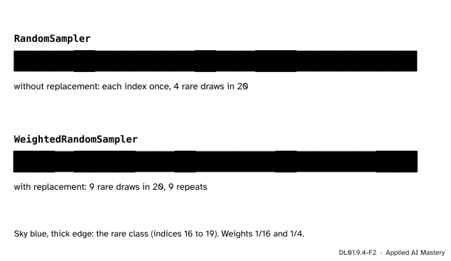
Step 4. Samplers. A sampler yields the indices a loader fetches. RandomSampler, which shuffle=True uses, yields each index once per epoch in a random order. WeightedRandomSampler draws indices with probabilities proportional to given weights, with replacement by default, so some indices come up several times and others not at all.
DL01.9.4-F2
Two samplers on 20 examples, 4 of them rare. With weights 1/16 for the common class and 1/4 for the rare one, each class is drawn half the time, so the rare examples come up again and again.
Step 5. Class weights. The other way leaves the sampler alone and changes the loss: nn.CrossEntropyLoss(weight=w) multiplies the loss of each example by the weight of its class, so a rare example counts more each time it is seen.
The formal statement
Stratified split. For each class \(k\) with \(n_k\) examples, a stratified split with test share \(t\) puts close to \(t\,n_k\) of them in the test part. Counts must be whole numbers, so scikit-learn rounds each class up or down in a way that makes the total exactly \(\lceil t\,n \rceil\).
The weighted sampler. Let \(K\) be the number of classes, \(n_k\) the number of training examples of class \(k\), and give example \(i\) the weight \(w_i = 1/n_{y_i}\). A WeightedRandomSampler draws \(i\) with probability \(w_i / \sum_j w_j\). The weights of class \(k\) add up to \({n_k \cdot (1/n_k)} = 1\), so \(\sum_j w_j = K\), and
Every class is drawn equally often, whatever its size.
Class weights in the loss. With a weight \(c_k\) for class \(k\), PyTorch’s weighted cross-entropy with the default reduction="mean" divides by the total weight of the batch, not by its size:
where \(\ell_i\) is the cross-entropy of example \(i\). Over the whole training set, class \(k\) carries total weight \(n_k c_k\). The choice \(c_k = {n / (K n_k)}\) makes that \(n/K\) for every class: each class weighs a \(K\)-th of the loss. The factor \(n/K\) only sets the scale; a weight is about one for a class of average size.
The same aim, two kinds of noise. Both remedies make each class count equally on average. The sampler does it by repetition: an epoch of \(n\) draws visits a rare image about \({n/(K n_k)}\) times. The class weights do it by size: every image comes once per epoch, but a rare one moves the gradient \(c_k\) times as much. Using both at once counts the rare class twice over.
Worked example
The split, class by class. Class 0 has 178 images. The test cut takes \({0.2 \cdot 178} = 35.6\), rounded to 36, leaving 142. The validation cut takes \({0.25 \cdot 142} = 35.5\), which becomes 35 (the rounding is shared out so the total is 360), leaving 107 for training. Over all ten classes the parts come to 1,077, 360 and 360, with 104 to 109, 35 to 37 and 35 to 37 images per class.
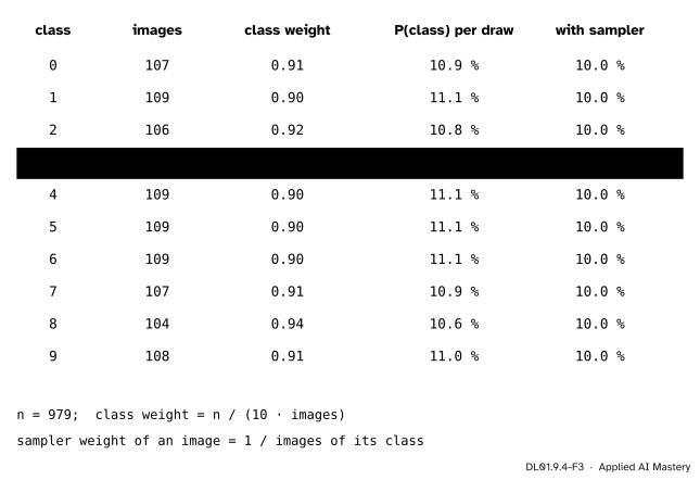
A class cut to a tenth. Keep only a tenth of the 109 training images of digit 3, rounded: 11. The training set shrinks to \({1077 - 109 + 11} = 979\) images.
DL01.9.4-F3
The training set with digit 3 cut to 11 images. Plain shuffling shows the network a 3 in about one draw of 90; the sampler in one draw of 10. The class weight of a 3 is 8.9.
Plain shuffling. Each epoch shows every image once, so a 3 is \({11/979} \approx 1.1\) percent of what the network sees.
The sampler. Weight \(1/11\) for each 3 and \(1/109\) for each 4, and so on. By the formula a draw is a 3 with probability \(1/10\), so an epoch of 979 draws holds about 98 threes, each of the 11 images about nine times.
The class weights.\(c_3 = {979 / (10 \cdot 11)} = 8.9\), and for digit 4, with 109 images, \(c_4 = 979/1090 \approx 0.898\). Total weight of the 3s: \({11 \cdot 8.9} = 97.9\), the same as for the 4s, \({109 \cdot 0.898} = 97.9\).
Code
The split, its class counts, and the indices kept for Subset.
import numpy as npimport torchimport torch.nn as nnfrom torch.utils.data import DataLoader, Subset, TensorDataset, WeightedRandomSampler, random_splitfrom sklearn.datasets import load_digitsfrom sklearn.model_selection import train_test_splitfrom sklearn.preprocessing import StandardScalertorch.manual_seed(0)torch.set_num_threads(1)digits = load_digits()y_all = digits.targetidx = np.arange(len(y_all))rest, test = train_test_split(idx, test_size=0.2, stratify=y_all, random_state=0)train, val = train_test_split(rest, test_size=0.25, stratify=y_all[rest], random_state=0)for name, part in (("train", train), ("val", val), ("test", test)): counts = np.bincount(y_all[part], minlength=10)print(f"{name:5}{len(part):5} per class {counts.min()} to {counts.max()}")full_set = TensorDataset(torch.tensor(digits.images.reshape(-1, 64) /16, dtype=torch.float32), torch.tensor(y_all))train_set, val_set = Subset(full_set, train), Subset(full_set, val)print(len(train_set), len(val_set), "class 0 in each part:", [int((y_all[p] ==0).sum()) for p in (train, val, test)])
train  1077  per class 104 to 109
val     360  per class 35 to 37
test    360  per class 35 to 37
1077 360 class 0 in each part: [107, 35, 36]
random_split against the stratified validation set, and how it rounds fractions.
parts = random_split(full_set, [1077, 360, 360], generator=torch.Generator().manual_seed(0))counts = np.bincount(y_all[parts[1].indices], minlength=10)print("random_split validation, per class:", counts.min(), "to", counts.max())print("fractions 0.6, 0.2, 0.2 give", [len(p) for p in random_split(full_set, [0.6, 0.2, 0.2], generator=torch.Generator().manual_seed(0))])
random_split validation, per class: 27 to 43
fractions 0.6, 0.2, 0.2 give [1079, 359, 359]
Scaling statistics come from the training set only. Five pixels are zero in every training image; a naive standardisation would divide by zero there, while StandardScaler leaves such a pixel unscaled.
X_train, X_val = full_set.tensors[0][train].numpy(), full_set.tensors[0][val].numpy()flat = np.flatnonzero(X_train.std(axis=0) ==0)scaler = StandardScaler().fit(X_train)print("pixels constant in training:", flat.tolist(), " their scale:", scaler.scale_[flat].tolist())print("validation images that light one of them:", int((X_val[:, flat] >0).any(axis=1).sum()))
pixels constant in training: [0, 24, 32, 39, 56]  their scale: [1.0, 1.0, 1.0, 1.0, 1.0]
validation images that light one of them: 1
Now cut digit 3 to a tenth and train the 64-32-10 network three ways, 20 epochs each with batches of 32 and lr=0.1: plain shuffling, the weighted sampler, and class weights in the loss.
X_tr, y_tr = full_set.tensors[0][train].numpy(), y_all[train]rng = np.random.default_rng(0)threes = np.flatnonzero(y_tr ==3)keep = np.sort(np.concatenate([np.flatnonzero(y_tr !=3), rng.choice(threes, size=round(len(threes) /10), replace=False)]))Xi, yi = torch.tensor(X_tr[keep]), torch.tensor(y_tr[keep])n_k = np.bincount(yi.numpy(), minlength=10)print("images:", len(yi), " of digit 3:", n_k[3], " class weight of 3:", round(len(yi) / (10* n_k[3]), 3))def train_and_score(mode, epochs=20): torch.manual_seed(0) model = nn.Sequential(nn.Linear(64, 32), nn.ReLU(), nn.Linear(32, 10)) data, gen = TensorDataset(Xi, yi), torch.Generator().manual_seed(0)if mode =="sampler": sampler = WeightedRandomSampler(torch.tensor(1.0/ n_k[yi.numpy()]), len(data), generator=gen) loader = DataLoader(data, batch_size=32, sampler=sampler)else: loader = DataLoader(data, batch_size=32, shuffle=True, generator=gen) weight = torch.tensor(len(yi) / (10* n_k), dtype=torch.float32) if mode =="weights"elseNone loss_fn, opt = nn.CrossEntropyLoss(weight=weight), torch.optim.SGD(model.parameters(), lr=0.1)for _ inrange(epochs):for xb, yb in loader: opt.zero_grad() loss_fn(model(xb), yb).backward() opt.step()with torch.no_grad(): pred = model(torch.tensor(X_val)).argmax(dim=1).numpy() y_v = y_all[val] recall = np.array([(pred[y_v == k] == k).mean() for k inrange(10)])return recall, (pred == y_v).mean()results = {mode: train_and_score(mode) for mode in ("plain", "sampler", "weights")}for mode, (recall, acc) in results.items():print(f"{mode:8} recall of 3: {recall[3]:.3f} lowest recall: {recall.min():.3f} accuracy: {acc:.3f}")
images: 979  of digit 3: 11  class weight of 3: 8.9
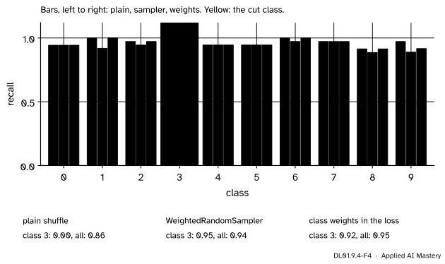
plain    recall of 3: 0.000   lowest recall: 0.000   accuracy: 0.864
sampler  recall of 3: 0.946   lowest recall: 0.886   accuracy: 0.936
weights  recall of 3: 0.919   lowest recall: 0.914   accuracy: 0.953
Two checks of the formal statement: the sampler draws digit 3 about a tenth of the time, and the weighted loss is the weighted mean of the per-example losses.
draws =list(WeightedRandomSampler(torch.tensor(1.0/ n_k[yi.numpy()]), 20*len(yi), generator=torch.Generator().manual_seed(0)))share = (yi.numpy()[draws] ==3).mean()logits, labels = torch.randn(6, 10, generator=torch.Generator().manual_seed(1)), torch.tensor([3, 3, 0, 1, 4, 9])c = torch.tensor(len(yi) / (10* n_k), dtype=torch.float32)by_hand = (c[labels] * nn.functional.cross_entropy(logits, labels, reduction="none")).sum() / c[labels].sum()print(f"share of 3s drawn: {share:.3f}; weighted loss {nn.CrossEntropyLoss(weight=c)(logits, labels).item():.4f}"f" = by hand {by_hand.item():.4f}")
share of 3s drawn: 0.102; weighted loss 2.1841 = by hand 2.1841
DL01.9.4-F4
Validation recall per class after training on the cut set. Plain shuffling recognises none of the 3s; both remedies recover most of them, at almost no cost to the other classes.
Explore
The epoch shuffler of DL01.9.3 uses a plain shuffled sampler on 24 tiles. Count how many times each tile appears in three epochs; then imagine a weighted sampler on the same tiles and say which counts would change. In the code above, try epochs=60 for the plain run and see whether more training alone rescues the 3s.
Pitfalls
DL01.9.4-F5
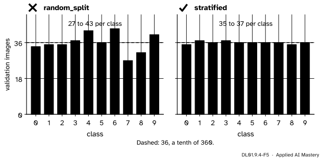
Wrong beside right. A random_split leaves the class mix to chance: from 27 to 43 validation images per class. The stratified split gives 35 to 37.
“random_split shuffles, so its parts are representative.”
Shuffling makes every split equally likely; it does not make any one split balanced. On a small or imbalanced set a rare class can be nearly missing from the validation set, and its recall is then estimated from a handful of images. Stratify with scikit-learn and wrap the indices in Subset.
“I copied the rare images ten times, then split.”
Copies of one image then land in both the training and the validation set, and the network is graded on images it has learned by heart: leakage (ML01.2.4). Split first, then oversample the training set only, which is what a WeightedRandomSampler does without making copies.
“Sampler and class weights together help twice as much.”
Each one on its own already makes the classes count equally. Together, the sampler already brings the 3s up to a tenth of the draws, and then each drawn 3 is weighted 8.9 against about 0.9 for any other digit. In the loss the 3s now weigh about ten times as much as any other digit, about half of the whole loss instead of a tenth, and the network is pushed to answer 3 whenever it is unsure. Use one remedy.
Check yourself
Recall
1. How are the 1,797 images split, and how large is each part?
Show answer
A stratified 20 percent test set (360), then a stratified quarter of the remaining 1,437 as validation (360), leaving 1,077 for training; both calls use random_state=0.
2. Why does random_split not keep the class mix?
Show answer
It cuts a random permutation of the indices by position and never looks at the labels.
3. With weights \(w_i = 1/n_{y_i}\), how often does a WeightedRandomSampler draw class \(k\)?
Show answer
With probability \(1/K\) per draw, whatever \(n_k\) is.
4. What does nn.CrossEntropyLoss(weight=c) divide by, with the default reduction?
Show answer
The total weight of the batch, \(\sum_{i \in B} c_{y_i}\), not the number of examples.
5. What is a Subset?
Show answer
A dataset made of another dataset and a list of indices into it; item \(j\) is item indices[j] of the original.
Exercises
1.★ Class 8 has 174 images. Follow it through both stratified cuts as in the worked example, and check the result against the counts in the code.
Show solution
Test: \({0.2 \cdot 174} = 34.8\), rounded to 35, leaving 139. Validation: \({0.25 \cdot 139} = 34.75\), rounded to 35, leaving 104 for training. The code reports 35, 35 and 104 for class 8: the smallest class sets the lower ends of the ranges, 104 and 35.
2.★★ A training set has 900 images of class A and 100 of class B. Find the WeightedRandomSampler weights and the class weights \(c_k = {n/(K n_k)}\), and the expected number of times each B image is drawn in an epoch of 1,000 draws.
Show solution
Sampler weights: \(1/900\) for each A image and \(1/100\) for each B image; each class is then drawn with probability \(1/2\). In 1,000 draws about 500 are B images, so each of the 100 is drawn about 5 times, and each A image about \({500/900} \approx 0.56\) times. Class weights: \(n = 1000\), \(K = 2\), so \(c_A = 1000/1800 \approx 0.556\) and \(c_B = 1000/200 = 5\); totals \({900 \cdot 0.556} = 500\) and \({100 \cdot 5} = 500\), equal.
3.★★★ Show that with class weights \(c_k\) and a batch drawn uniformly, the weighted mean loss over the whole training set gives each class the share \({n_k c_k / \sum_j n_j c_j}\), and that this share is \(1/K\) for every class exactly when \(c_k\) is proportional to \(1/n_k\).
Show solution
Over the whole set the weighted mean is \(\frac{\sum_i c_{y_i}\ell_i}{\sum_i c_{y_i}}\). Group the examples by class: the numerator is \(\sum_k c_k \sum_{i : y_i = k} \ell_i\) and the denominator \(\sum_k n_k c_k\). Class \(k\)’s examples together carry weight \(n_k c_k\) out of \(\sum_j n_j c_j\), which is its share. The shares are all equal, hence all \(1/K\), exactly when \(n_k c_k\) is the same number \(a\) for every class, that is when \(c_k = a / n_k\). The course’s choice \(c_k = {n/(K n_k)}\) is the case \(a = n/K\).
Summary card
Split by class, fix it once, then choose how the loader visits the training set.
DL01.9.4-F1
1,077, 360 and 360, stratified.
The split.train_test_split(..., test_size=0.2, stratify=y, random_state=0), then 0.25 of the rest.
PyTorch.random_split does not stratify; Subset(ds, indices) wraps your own split.
Sampler.\(w_i = 1/n_{y_i}\) draws each class with probability \(1/K\).
Class weights.\(c_k = {n/(K n_k)}\) gives each class total weight \(n/K\). Use one remedy, not both.
Sources and next steps
Sources. Each was opened and checked against this lesson on 15 November 2026.
scikit-learn 1.9 documentation, train_test_split: a float test_size is the proportion of the dataset in the test split; with stratify, the data is split in a stratified fashion using it as the class labels; random_state makes the shuffling reproducible. The rounding up of the test share was read in its source code and is checked by the cells above.
scikit-learn 1.9 documentation, StandardScaler: if a variance is zero, the data is left as it is, giving a scaling factor of 1.
PyTorch 2.15 documentation, torch.utils.data: random_split with lengths or fractions, remainders distributed one at a time in round-robin order; Subset as a dataset at specified indices; RandomSampler; WeightedRandomSampler samples from 0 to len(weights) - 1 with the given weights, which need not sum to one, with replacement by default.
PyTorch 2.15 documentation, torch.nn.CrossEntropyLoss: weight is a manual rescaling weight given to each class, and with the mean reduction the weighted losses are divided by the sum of the weights of the targets.
Next. DL01.10, First project: an image classifier, takes this split and these loaders and trains the 64-32-10 network for real.