Wrap the five lines in an outer loop: an epoch over the training data, a validation pass under torch.no_grad() and model.eval(), epoch metrics weighted by batch size, and training curves drawn from a history dictionary.
DL01.8.2L2 Intermediate25 minIn review (what this means)
The maths and code on this page are checked by automated tests on every change, but an independent reader has not signed it off yet. Spot a mistake or a confusing step? Tell us.
Write a train_one_epoch and an evaluate function and combine them into an epoch loop with a history.
Compute an epoch’s loss and accuracy as averages weighted by batch size, and show why the plain mean of batch means is wrong.
Explain what model.train(), model.eval() and torch.no_grad() each switch, and why they are independent.
Explain why the training loss averaged over an epoch differs from the loss of the weights at its end.
The question
After one iteration the network is a little better on one batch. But is it better at the task, on points it has never trained on? To answer that you need a second loop around the first, a regular check on data the updates never touch, and two switches that most training scripts flip without saying why. What do they switch, and how should the numbers of an epoch be added up?
From the last lesson
1. What does loss.backward() do to a parameter’s .grad?
Show answer
It adds the partial derivative of the loss into .grad; it does not overwrite it. Then it frees the graph.
2. In the worked example of DL01.8.1, what did .grad hold at step 2 when zero_grad was forgotten?
Show answer
\({(-23.5, -8)}\) plus \({(-3.875, -1.325)}\), which is \({(-27.375, -9.325)}\): step 1’s gradient plus step 2’s.
Intuition
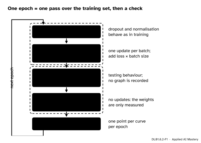
An epoch is one pass over the whole training set, batch by batch, with one update per batch. After each epoch the loop stops learning for a moment and measures: it runs the network on the validation set, the points set aside to estimate how well the network does on data it was not fitted to (ML01.2), and it writes the numbers down.
DL01.8.2-F1
One epoch: a training pass that updates the weights, then a validation pass that only measures them, then one new point on each curve.
The two halves of the epoch differ in three ways. The training pass updates the weights; the validation pass must not. The training pass needs the computational graph for backward; the validation pass does not, so recording it would waste memory and time. And some layers, which this course meets in DL02, are meant to behave differently while training and while being tested. Each difference has its own switch.
Build it up
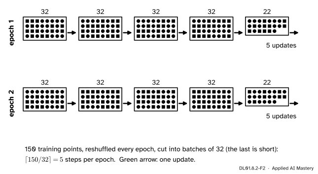
Step 1. Batches. A data loader hands out the training set in batches. Here it is PyTorch’s DataLoader over the 150 training points with batch_size=32 and shuffle=True; DL01.9 opens it up and builds one from scratch. With 150 points and batches of 32, an epoch has \({\lceil 150 / 32 \rceil = 5}\) steps: four batches of 32 and a short last batch of 22.
DL01.8.2-F2
An epoch of the make_moons training set. The points are reshuffled every epoch and cut into batches of 32, so the last batch is short.
Step 2. The training pass. Call model.train(), then run the five lines on every batch. Keep a running total of loss.item() times the batch size and of the number of correct predictions, so that the epoch’s numbers can be computed at the end.
Step 3. The validation pass. Call model.eval() and wrap the pass in with torch.no_grad():. Run only the forward pass and the loss on each validation batch. There is no zero_grad, no backward and no step: the weights are measured, not changed.
Step 4. The history. Append the epoch’s training loss, validation loss and validation accuracy to the lists of a dictionary. After training, each list is a curve to draw, one point per epoch.
The formal statement
NoteEpoch metrics
An epoch splits the \(n\) training examples into batches \(B_1, \dots, B_m\) that do not overlap and cover every example once, with \({m = \lceil n/B \rceil}\) for batch size \(B\). If \(L_k\) is the mean loss on batch \(k\), the epoch loss is the average weighted by batch size:
\[
\bar L = \frac{1}{n} \sum_{k=1}^{m} \abs{B_k}\, L_k .
\]
Why this is the mean over examples. Write \(\ell_i\) for the loss of example \(i\). A batch mean is \({L_k = \frac{1}{\abs{B_k}} \sum_{i \in B_k} \ell_i}\), so \({\abs{B_k} L_k = \sum_{i \in B_k} \ell_i}\). The batches cover every example exactly once, so
The same argument holds for accuracy, with \(\ell_i\) replaced by 1 for a correct prediction and 0 otherwise. The plain mean \({\frac1m \sum_k L_k}\) gives every batch the weight \(1/m\) instead of \(\abs{B_k}/n\). The two agree when all batches have the same size and differ when the last one is short.
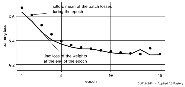
The epoch’s training loss is a blend of \(m\) networks. The batch losses are recorded during the epoch, each just before its update. So \(L_1\) belongs to the weights at the start of the epoch, \(L_2\) to the weights after one update, and so on. The validation loss is measured once, at the end. Early in training, when the loss falls quickly, the running average therefore sits above the loss of the end-of-epoch weights.
DL01.8.2-F4
The training loss averaged during each epoch (circles) against the loss of the weights reached at the end of it (line). The gap is largest while the loss falls fastest.
The two switches.
model.train() and model.eval() set a flag, training, on the model and every layer inside it. Only some layers read it. Dropout (DL02.5) in training mode multiplies each value \(a\) by a random \({m / (1 - p)}\), where \(m\) is 0 with probability \(p\) and 1 otherwise. Since \({\E[m] = 1 - p}\), the expected output is \({(1 - p)\, a / (1 - p)}\), which is \(a\), so in evaluation mode it can simply pass \(a\) through. Batch normalisation (DL02.6) uses the batch’s own statistics in training mode and stored ones in evaluation mode.
torch.no_grad() stops autograd from recording the graph. Outputs computed inside it have requires_grad=False, and no activations are kept for a backward pass.
They are independent. The PyTorch notes say that evaluation mode “is not a mechanism to locally disable gradient computation”, and no_grad does not change how dropout behaves. The validation pass needs both. The 2-16-16-2 network has no dropout or normalisation, so for it model.eval() changes nothing yet. The loop calls it anyway, because the same code will train networks that do.
Worked example
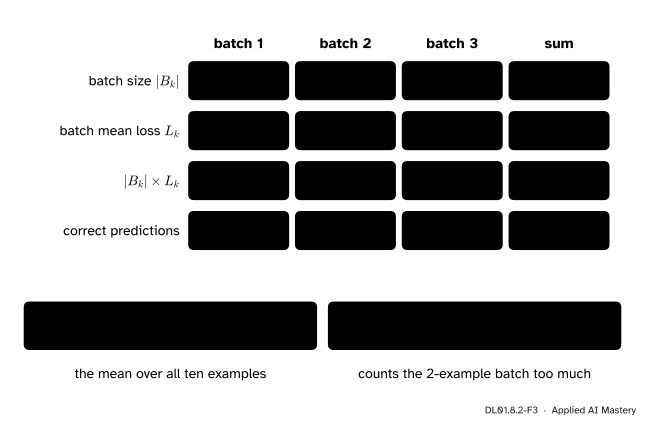
Ten training examples are cut into batches of 4, 4 and 2. The batch mean losses are 0.6, 0.5 and 0.2, and the batches get 3, 3 and 2 predictions right.
Weighted. Multiply each batch mean by its size: \({4 \cdot 0.6 = 2.4}\), \({4 \cdot 0.5 = 2.0}\) and \({2 \cdot 0.2 = 0.4}\). These are the sums of the per-example losses in each batch. Their total is 4.8, so the epoch loss is \({4.8 / 10 = 0.48}\). The correct predictions add to 8, so the accuracy is \({8 / 10 = 0.80}\).
Plain mean.\({(0.6 + 0.5 + 0.2)/3 = 1.3/3 \approx 0.433}\), and the mean of the batch accuracies \({(0.75 + 0.75 + 1)/3 \approx 0.833}\). Both are wrong. The short batch, which happens to have low loss and no mistakes, counts as a third of the epoch although it holds a fifth of the examples.
DL01.8.2-F3
The worked example as a trace. Weighting by batch size recovers the mean over the ten examples.
The error of the plain mean is \({\sum_k (\tfrac13 - \tfrac{\abs{B_k}}{10}) L_k}\). The weights differ by \({\tfrac13 - \tfrac{4}{10} = -\tfrac{1}{15}}\) for the full batches and \({\tfrac13 - \tfrac{2}{10} = \tfrac{2}{15}}\) for the short one, so
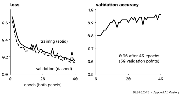
epoch  1: train loss 0.671  val loss 0.622  val acc 0.80
epoch 10: train loss 0.310  val loss 0.267  val acc 0.90
epoch 20: train loss 0.265  val loss 0.268  val acc 0.90
epoch 40: train loss 0.147  val loss 0.126  val acc 0.96
The weighted validation loss equals the loss on all 50 points at once; the plain mean of the two batch losses does not. And the two switches do what the formal statement says.
X_all, y_all = val_set.tensorswith torch.no_grad(): whole = loss_fn(model(X_all), y_all).item() batch_means = [loss_fn(model(X), y).item() for X, y in val_loader]print(f"all 50 at once {whole:.6f}, weighted {evaluate(model, loss_fn, val_loader)[0]:.6f}, "f"plain mean {np.mean(batch_means):.6f}")model.train(); out_train = model(X_all)model.eval(); out_eval = model(X_all)with torch.no_grad(): out_quiet = model(X_all)print("train and eval outputs equal:", torch.equal(out_train, out_eval))print("requires_grad outside / inside no_grad:", out_eval.requires_grad, out_quiet.requires_grad)torch.manual_seed(0)drop = nn.Dropout(p=0.5)ones = torch.ones(8)print("dropout, train mode:", drop(ones).tolist())drop.eval()print("dropout, eval mode: ", drop(ones).tolist())
all 50 at once 0.125688, weighted 0.125688, plain mean 0.110017
train and eval outputs equal: True
requires_grad outside / inside no_grad: True False
dropout, train mode: [0.0, 0.0, 2.0, 0.0, 0.0, 0.0, 2.0, 2.0]
dropout, eval mode:  [1.0, 1.0, 1.0, 1.0, 1.0, 1.0, 1.0, 1.0]
In training mode dropout zeroes about half of the ones and doubles the rest, \({1/(1 - 0.5) = 2}\); in evaluation mode it passes them through.
Explore
DL01.8.2-F5
The history of the run above, drawn as curves. Validation loss is dashed, as everywhere in the course.
The loop stepper of DL01.8.1 runs the inner loop one line at a time. Here, read the curves: both losses fall together, and the validation accuracy climbs in steps of 0.02 because each of the 50 validation points is worth that much. DL01.8.3 reads curves that go wrong.
Pitfalls
DL01.8.2-F6
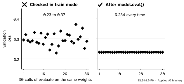
Wrong beside right on a make_moons network with dropout. In training mode each check of the same weights gives a different validation loss. After model.eval() the check is a measurement.
“No step is taken during validation, so the mode does not matter.”
Dropout stays random in training mode, so the same weights score anywhere from about 0.23 to 0.37 in the figure, and a normalisation layer in training mode would even blend the statistics of the validation batches into its stored ones, no_grad or not. Call model.eval() before validating and model.train() before the next training pass.
“torch.no_grad() puts the model in evaluation mode.”
It only stops the graph from being recorded. Dropout and normalisation read the training flag, which only train() and eval() change. The validation pass needs both switches.
“The epoch loss is the mean of the batch losses,” or “total_loss += loss is fine.”
The first gives a short last batch too much weight: multiply by the batch size and divide by the number of examples. The second adds the loss tensor, so the total carries the computation history of every batch, and memory grows through the epoch. Add loss.item(), a plain number.
Check yourself
Recall
1. How many steps does an epoch of 150 examples in batches of 32 take, and what sizes are the batches?
Show answer
\({\lceil 150/32 \rceil = 5}\) steps: four batches of 32 and a last batch of 22.
2. Write the epoch loss in terms of the batch means \(L_k\) and batch sizes \(\abs{B_k}\).
Show answer
\({\bar L = \frac1n \sum_k \abs{B_k} L_k}\), which equals the mean loss over all \(n\) examples.
3. What does model.eval() change, and what does torch.no_grad() change?
Show answer
eval() sets the training flag to false, which changes how dropout and normalisation layers behave. no_grad() stops autograd from recording the graph. They are independent.
4. In training mode with \({p = 0.5}\), what does dropout do to a value of 1, and why is the expected output still 1?
Show answer
It becomes 0 with probability 0.5 and \({1/(1 - 0.5) = 2}\) otherwise. The expectation is \({0.5 \cdot 0 + 0.5 \cdot 2 = 1}\).
5. Why does the training loss averaged during an epoch usually sit above the loss of the weights at the end of that epoch, early in training?
Show answer
Each batch loss is recorded before its update, with the weights of that moment. The average mixes older weights, which were worse while the loss was falling.
Exercises
1.★ An epoch of 1,077 images (DL01.9’s training set) runs in batches of 64. How many steps does it take, how big is the last batch, and with what weight should the last batch’s mean loss enter the epoch loss?
Show solution
\({1077 = 16 \cdot 64 + 53}\), so \({\lceil 1077/64 \rceil = 17}\) steps, sixteen batches of 64 and a last batch of 53. Its mean loss enters with weight \({53/1077 \approx 0.0492}\), against \({64/1077 \approx 0.0594}\) for each full batch. The plain mean would give every batch \({1/17 \approx 0.0588}\).
2.★★ Batches of sizes 32, 32, 32, 32 and 22 have mean losses 0.40, 0.38, 0.36, 0.35 and 0.10. Find the weighted epoch loss and the plain mean, and say which batch causes the difference.
Show solution
The products are \({32 \cdot 0.40 = 12.8}\), \({32 \cdot 0.38 = 12.16}\), \({32 \cdot 0.36 = 11.52}\), \({32 \cdot 0.35 = 11.2}\) and \({22 \cdot 0.10 = 2.2}\). Their sum is 49.88, so the epoch loss is \({49.88/150 \approx 0.3325}\). The plain mean is \({1.59/5 = 0.318}\). The short last batch, with an unusually low loss, gets weight \({1/5 = 0.2}\) in the plain mean instead of \({22/150 \approx 0.147}\), which pulls the plain mean down.
3.★★★ A dropout layer with probability \(p\) acts on a value \(a\). Find the mean and the variance of its output in training mode, and say what the variance means for a validation loss measured in training mode.
Show solution
The output is \({X = m a/(1 - p)}\), with \({m = 1}\) with probability \({1 - p}\) and 0 otherwise. Then
For \({p = 0.5}\) that is \(a^2\): the standard deviation equals the value itself. Every hidden value is that noisy, so a validation loss measured in training mode is a random number, not a property of the weights, as the pitfall figure shows. In evaluation mode the variance is zero.
Summary card
An epoch trains on every batch once, then measures on validation without touching the weights.
DL01.8.2-F1
Train, then measure, then record.
Steps per epoch: \({\lceil n/B \rceil}\); the last batch may be short.
Epoch loss: \({\bar L = \frac1n \sum_k \abs{B_k} L_k}\), the mean over examples.
model.eval() changes layer behaviour; torch.no_grad() stops the graph. Validate with both.
Add loss.item(), never the loss tensor, to a running total.
Sources and next steps
Sources. Each was opened and checked against this lesson on 15 November 2026.
Simon J. D. Prince, Understanding Deep Learning (MIT Press, 2023), section 6.2.1: batches are drawn without replacement until all the data have been used, and a single pass through the training set is an epoch.
PyTorch 2.15 documentation, Autograd mechanics, sections “No-grad mode” and “Evaluation mode”: computations in no-grad mode behave as if no input requires grad, and evaluation mode “is not a mechanism to locally disable gradient computation”.
PyTorch 2.15 documentation, torch.nn.Module: train() and eval() affect only certain modules, such as Dropout and BatchNorm, and eval() is equivalent to train(False); and torch.nn.Dropout: zeroes elements with probability \(p\) in training, scales the rest by \({1/(1 - p)}\), and is the identity in evaluation.
PyTorch 2.15 documentation, Frequently asked questions, “Don’t accumulate history across your training loop”: total_loss += loss keeps history; write total_loss += float(loss).