Stack the examples as rows and the backward pass becomes three matrix products per layer: vector-Jacobian products that never form a Jacobian. Derive the batch rules, check every shape, then train the XOR network with a few hundred steps of gradient descent.
M05.9.2L2 Intermediate25 minIn review (what this means)
The maths and code on this page are checked by automated tests on every change, but an independent reader has not signed it off yet. Spot a mistake or a confusing step? Tell us.
Write the forward and backward pass of a stack of dense tanh layers for a whole batch as matrix products, with the shape of every matrix.
Derive the batch rules for the weight gradient, the bias gradient and the adjoint of the layer below from the dense-layer rules of M05.7.3.
Explain why backpropagation multiplies by Jacobians without ever forming them, and count what forming them would cost.
Implement batch backpropagation in NumPy and train the XOR network with gradient descent.
The question
A digit classifier with 784 inputs, 100 hidden units and 10 outputs sees a batch of 64 images at a time. The Jacobian of its 640 output scores with respect to its first weight matrix alone has about 50 million entries. Libraries compute the gradient of the loss for every one of its 79,510 parameters in a few matrix products. Which products, and why is no Jacobian ever needed?
From the last lesson
1. For a sigmoid output with the log loss, what is the adjoint of the output score?
Show answer
\({\delta^{(2)} = p - y}\).
2. How does an adjoint pass through a tanh layer?
Show answer
Entry by entry, times \({1 - a^2}\) at each unit.
Intuition
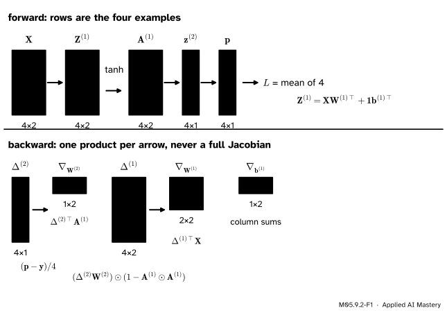
Lesson M05.9.1 ran backpropagation on one example. A batch is the same thing done for every example at once: put the examples in the rows of a matrix, and every vector of the last lesson becomes a matrix with one row per example. Each arrow of the backward pass is then one matrix product.
M05.9.2-F1
The whole batch at once. Every forward quantity is a matrix with one row per example; every backward quantity is a matrix product or an entrywise product, and each gradient has the shape of the thing it belongs to.
Two things make this cheap. First, a dense layer passes adjoints back with a product by its weight matrix, so the Jacobian of the layer is used but never written down. Second, an elementwise activation has a diagonal Jacobian, and multiplying by a diagonal matrix is an entrywise product. Each step is a vector-Jacobian product: a row of adjoints times a Jacobian, done without the Jacobian.
Build it up
Step 1. Rows are examples. Stack the inputs as the rows of \(\cdata{\mat{X}}\), \({n \times 2}\) for XOR with \({n = 4}\). Example \(i\) has \({\vect{z}^{(1)}_i} = {\mat{W}^{(1)}\vect{x}_i} + {\vect{b}^{(1)}}\), and its transpose is a row: \({\vect{x}_i\T\mat{W}^{(1)\top}} + {\vect{b}^{(1)\top}}\). Stacking the rows,
where \(\vect{1}\) is a column of \(n\) ones. This is the batch layer \({\mat{Y}} = {\mat{X}\mat{W}} + {\vect{1}\vect{b}\T}\) of M05.7.3, with its weight matrix equal to \({\mat{W}^{(1)\top}}\).
Step 2. The mean loss.\({L = \frac{1}{n}\sum_i \ell_i}\), so a change in example \(i\)’s score changes \(L\) by \(\frac{1}{n}\) of what it changes \(\ell_i\). The output adjoints form a column, \({\mat{\Delta}^{(2)}} = {(\vect{p} - \vect{y})/n}\), one entry per example.
Step 3. Back through a dense layer. Given the adjoint \(\mat{G}\) of a layer’s output, M05.7.3 gave \({\nabla_{\mat{W}}L} = {\mat{X}\T\mat{G}}\) and \({\nabla_{\mat{X}}L} = {\mat{G}\mat{W}\T}\) for \({\mat{Y}} = {\mat{X}\mat{W}} + {\vect{1}\vect{b}\T}\). Our layer’s weight matrix is \({\mat{W}^{(l)\top}}\), so transpose the first rule and drop the double transpose in the second: \({\nabla_{\mat{W}^{(l)}}L} = {\mat{G}\T\mat{A}^{(l-1)}}\) and \({\partial L/\partial\mat{A}^{(l-1)}} = {\mat{G}\,\mat{W}^{(l)}}\).
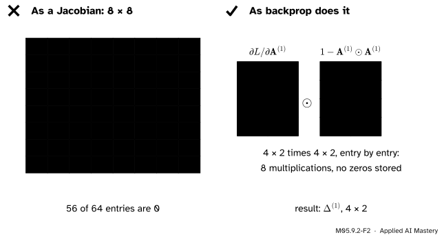
Step 4. Through the activation.\({\mat{A} = \tanh\mat{Z}}\) entry by entry, so its Jacobian, for the whole batch, is a diagonal matrix with one entry per number in \(\mat{Z}\). Multiplying by it is the entrywise product with \({1 - \mat{A} \odot \mat{A}}\).
M05.9.2-F2
The tanh layer of the XOR batch. As a Jacobian it is an \({8 \times 8}\) matrix that is almost all zeros; backpropagation uses only its diagonal, laid out in the shape of \(\mat{Z}^{(1)}\), and multiplies entry by entry.
Step 5. Nothing else. Weight gradient, adjoint of the layer below, activation: repeated from the top layer down, these three products are the whole backward pass.
The formal statement
NoteBackpropagation for a batch
Take layers \({\mat{Z}^{(l)}} = {\mat{A}^{(l-1)}\mat{W}^{(l)\top}} + {\vect{1}\vect{b}^{(l)\top}}\) for \({l = 1, \dots, K}\), with \({\mat{A}^{(0)} = \mat{X}}\), \({\mat{A}^{(l)} = \tanh\mat{Z}^{(l)}}\) for the hidden layers, a sigmoid output \({\vect{p} = \sigma(\mat{Z}^{(K)})}\) and the mean log loss over \(n\) examples. Let \(\mat{\Delta}^{(l)}\) be the adjoint of \(\mat{Z}^{(l)}\). Then
the last for \({l = K, \dots, 2}\). Row \(i\) of \(\mat{\Delta}^{(l)}\) is \({\vect{\delta}^{(l)}_i/n}\), the per-example adjoint of M05.9.1 divided by \(n\).
Derivation. The output line is Step 2 with the result \({\delta = p - y}\) of M05.9.1 for each example. The weight and bias lines are Step 3: the bias gradient \({\mat{G}\T\vect{1}}\) is from M05.7.3 unchanged, and it adds up the column of each output unit. The last line is Step 3’s \({\partial L/\partial\mat{A}^{(l-1)}} = {\mat{\Delta}^{(l)}\mat{W}^{(l)}}\) followed by Step 4.
To see that this is the per-example rule of M05.9.1, look at one row. Row \(i\) of \({\mat{\Delta}^{(l)}\mat{W}^{(l)}}\) is \({(\vect{\delta}^{(l)}_i/n)\T\mat{W}^{(l)}}\), the transpose of \({\mat{W}^{(l)\top}\vect{\delta}^{(l)}_i/n}\): exactly the column rule \({\vect{\delta}^{(l-1)}} = {(\mat{W}^{(l)\top}\vect{\delta}^{(l)}) \odot \tanh'(\vect{z}^{(l-1)})}\), one example per row. And a product \({\mat{B}\T\mat{C}}\) is the sum over rows \(i\) of the outer products \({\vect{b}_i\vect{c}_i\T}\), so
the mean of the per-example gradients of M05.9.1. The batch rules are the per-example rules, summed by matrix multiplication.
Shapes. Every gradient has the shape of its parameter, and every adjoint the shape of its value. For the XOR batch and for a digit classifier with a softmax output (where M05.7.3 gives \({\mat{\Delta}^{(2)}} = {(\mat{P} - \mat{T})/B}\) for the targets \(\mat{T}\)):
What a Jacobian would cost. The Jacobian of the 640 output scores with respect to the 78,400 entries of \(\mat{W}^{(1)}\) has \({640 \times 78{,}400} = {50{,}176{,}000}\) entries. Backpropagation instead multiplies \({\mat{\Delta}^{(1)\top}}\), a \({100 \times 64}\) matrix, by the \({64 \times 784}\) input: \({100 \times 64 \times 784}\), about five million multiply-adds, with an answer the size of the weights. This is reverse mode’s left-to-right order (M05.8.4): a row of adjoints times each Jacobian in turn, never a Jacobian times a Jacobian.
Worked example
The XOR batch at the starting weights. Every number is rounded from an unrounded computation, so redoing a sum with the rounded values can change its last digit. Forward, by the rows of M05.9.1:
\({\vect{p}} \approx {(0.5,\ 0.121,\ 0.743,\ 0.318)}\) and the mean loss is \({(0.693 + 2.114 + 0.297 + 0.383)/4} \approx {0.872}\).
Output.\({\mat{\Delta}^{(2)}} = {(\vect{p} - \vect{y})/4} \approx {(0.125,\ -0.220,\ -0.064,\ 0.080)}\), a column. Its sum is the bias gradient, \({\partial L/\partial b^{(2)}} \approx {-0.080}\).
Second layer.\({\mat{\Delta}^{(2)\top}\mat{A}^{(1)}}\) is a row of two dot products. The first is \({0.125 \cdot 0} + {(-0.220)(-0.762)} + {(-0.064)(0.762)} + {0.080 \cdot 0}\), which comes to about 0.118. The second, with the second column of \(\mat{A}^{(1)}\), comes to about \(-0.071\). So \({\nabla_{\mat{W}^{(2)}}L} \approx {(0.118,\ -0.071)}\).
Hidden adjoints.\({\mat{\Delta}^{(2)}\mat{W}^{(2)}}\) puts \({2\Delta^{(2)}_i}\) and \({-\Delta^{(2)}_i}\) in row \(i\); the entrywise product with \({1 - \mat{A}^{(1)} \odot \mat{A}^{(1)}}\) gives
Row 2 is \({(-0.739,\ 0.691)/4}\), the adjoint of M05.9.1 divided by \(n\). The column sums give \({\nabla_{\vect{b}^{(1)}}L} \approx {(0.171,\ 0.065)}\).
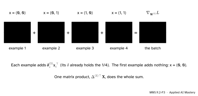
First layer.\({\mat{\Delta}^{(1)\top}\mat{X}}\) adds the outer products \({\vect{\delta}_i\vect{x}_i\T}\) (with the \(\frac{1}{4}\) inside \(\vect{\delta}_i\)):
M05.9.2-F3
The gradient of \(\mat{W}^{(1)}\) as the sum of one outer product per example. An input of 0 wipes out a column, so the example \({(0, 0)}\) contributes nothing to \(\mat{W}^{(1)}\), though it has the largest adjoint.
From scratch: forward and backward passes for any stack of dense tanh layers with a sigmoid output and the mean log loss. A list of (W, b) pairs describes the network, so the same code serves a 2-2-1 or a 784-100-10 network.
import numpy as npdef forward(layers, X):"""Return the activations A0 = X, A1, ..., and the output probabilities.""" A = [X]for l, (W, b) inenumerate(layers): Z = A[-1] @ W.T + b # rows are examples A.append(np.tanh(Z) if l <len(layers) -1else1/ (1+ np.exp(-Z)))return Adef mean_log_loss(layers, X, y): p = forward(layers, X)[-1][:, 0]return-np.mean(y * np.log(p) + (1- y) * np.log(1- p))def backward(layers, X, y):"""Gradients of the mean log loss, as a list of (grad W, grad b) pairs, one per layer.""" A = forward(layers, X) Delta = (A[-1] - y[:, None]) /len(y) # adjoint of the output scores, n x 1 grads = [None] *len(layers)for l inreversed(range(len(layers))): W, b = layers[l] grads[l] = (Delta.T @ A[l], Delta.sum(axis=0))if l >0: Delta = (Delta @ W) * (1- A[l] **2) # adjoint of the layer belowreturn gradsX = np.array([[0.0, 0.0], [0.0, 1.0], [1.0, 0.0], [1.0, 1.0]])y = np.array([0.0, 1.0, 1.0, 0.0])start = [(np.array([[1.0, -1.0], [0.5, 0.5]]), np.zeros(2)), (np.array([[2.0, -1.0]]), np.zeros(1))](gW1, gb1), (gW2, gb2) = backward(start, X, y)print(f"loss = {mean_log_loss(start, X, y):.3f}")print("grad W1 =", np.round(gW1, 3).tolist(), " grad b1 =", np.round(gb1, 3).tolist())print("grad W2 =", np.round(gW2, 3).tolist(), " grad b2 =", np.round(gb2, 3).tolist())
loss = 0.872
grad W1 = [[0.105, -0.025], [0.017, 0.139]]  grad b1 = [0.171, 0.065]
grad W2 = [[0.118, -0.071]]  grad b2 = [-0.08]
The batch gradient should be the mean of the four per-example gradients of M05.9.1, and should agree with central differences. Both checks, on every parameter:
per_example = [backward(start, X[i:i +1], y[i:i +1])[0][0] for i inrange(4)]print("mean of per-example grad W1 equals the batch grad:", np.allclose(np.mean(per_example, axis=0), gW1))def numeric(layers, h=1e-5): out = []for W, b in layers:for P in (W, b): G = np.zeros_like(P)for idx in np.ndindex(P.shape): old = P[idx] P[idx] = old + h; up = mean_log_loss(layers, X, y) P[idx] = old - h; down = mean_log_loss(layers, X, y) P[idx] = old G[idx] = (up - down) / (2* h) out.append(G)return outflat_backprop = np.concatenate([g.ravel() for pair in backward(start, X, y) for g in pair])flat_numeric = np.concatenate([g.ravel() for g in numeric(start)])gap = np.linalg.norm(flat_backprop - flat_numeric) / (np.linalg.norm(flat_backprop) + np.linalg.norm(flat_numeric))print(f"relative error against central differences: {gap:.1e}")
mean of per-example grad W1 equals the batch grad: True
relative error against central differences: 4.6e-11
Now train. Gradient descent (ML01.5.2) moves every parameter against its gradient, \({\theta \leftarrow \theta - \eta\,\nabla L}\); with \({\eta = 1}\), a rate found by trying a few (ML01.5.3), 300 full-batch steps:
layers = [(W.copy(), b.copy()) for W, b in start]history = [mean_log_loss(layers, X, y)]for step inrange(300): grads = backward(layers, X, y) layers = [(W -1.0* gW, b -1.0* gb) for (W, b), (gW, gb) inzip(layers, grads)] history.append(mean_log_loss(layers, X, y))p_final = forward(layers, X)[-1][:, 0]print("loss at steps 0, 50, 100, 300:", [round(float(history[k]), 3) for k in (0, 50, 100, 300)])print("predicted probabilities:", np.round(p_final, 3), " labels:", y)
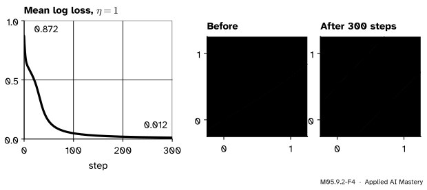
The loss falls from 0.872 to about 0.012, and the network now puts all four points on the right side of \({p = 1/2}\). Training practice, mini-batches and better optimisers are DL01.8 and DL02.1.
M05.9.2-F4
Training the running network. The loss curve is the output of the cell above; the decision maps show where the network says \({p > 1/2}\) (darker) before and after. A straight line cannot separate XOR; the hidden layer bends the boundary into a band.
Explore
M05.9-X1
Backprop stepper
Choose one example or the whole batch and press Step: the forward pass fills the nodes with values, then the backward pass fills them with adjoints and the table with weight gradients, each beside its central-difference check. Then set the learning rate and train.
Three things to try. Choose the example \({(0, 1)}\) and step to the end: the table shows the numbers of M05.9.1. Choose the batch and compare the table with the worked example above. Then train with \({\eta = 1}\): the loss falls below 0.05 within about a hundred steps and the band of the decision map opens up. Try \({\eta = 0.1}\), where the loss is still near 0.59 after a hundred steps, and \({\eta = 5}\), where it jumps up and down before it settles lower than with \({\eta = 1}\).
Pitfalls
M05.9.2-F5
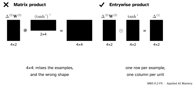
Wrong beside right. The activation’s Jacobian is diagonal, so it enters as an entrywise product of two matrices of the same shape. A matrix product mixes different examples and gives a \({4 \times 4}\) result.
“tanh’ is a matrix, so multiply by it.”
It is a diagonal matrix, and a diagonal matrix acts entry by entry. Written as (Delta @ W) @ D.T the product is \({n \times n}\); when the batch size equals the layer width that is the expected shape, the code runs, and it silently mixes examples. Write (Delta @ W) * D, and assert that every adjoint has the shape of its value.
“The bias gradient is the adjoint matrix.”
\(\mat{\Delta}^{(l)}\) has one row per example; the bias has one entry per unit. Its gradient is the column sum \({\mat{\Delta}^{(l)\top}\vect{1}}\), because the same bias is added to every row, and a value used in several places collects the sum of its adjoints.
“Build each layer’s Jacobian, then multiply them.”
For the digit classifier a single such Jacobian has about 50 million entries, and multiplying Jacobians together is forward mode’s expensive order. Backpropagation needs only products of a row of adjoints with each Jacobian, and each of those is a matrix product the size of the layer.
Check yourself
Recall
1. In the batch layout, what does a row of \(\mat{Z}^{(l)}\) hold?
Show answer
The pre-activations of layer \(l\) for one example.
2. What is the gradient of \(\mat{W}^{(l)}\) for a batch?
Show answer
\({\mat{\Delta}^{(l)\top}\mat{A}^{(l-1)}}\): the sum over examples of the outer products of their adjoints and inputs.
3. How is the adjoint passed to the layer below?
Show answer
Multiply \({\mat{\Delta}^{(l)}\mat{W}^{(l)}}\) entry by entry by \({1 - \mat{A}^{(l-1)} \odot \mat{A}^{(l-1)}}\) for tanh units; the result is \({\mat{\Delta}^{(l-1)}}\).
4. Where does the factor \(1/n\) of the mean loss enter?
Show answer
Once, in the output adjoint \({(\vect{p} - \vect{y})/n}\); every later product carries it along.
5. Why is no Jacobian ever formed?
Show answer
Each step only needs a row of adjoints times a Jacobian, a vector-Jacobian product, which for a dense layer is a product with the weight matrix and for an activation an entrywise product.
Exercises
1.★ A network 10-5-3-1 (two tanh hidden layers, one sigmoid output) is trained on batches of 8. Give the shapes of \(\mat{X}\), of every weight matrix, and of every \(\mat{\Delta}^{(l)}\).
Show solution
\(\mat{X}\) is \({8 \times 10}\). \(\mat{W}^{(1)}\) is \({5 \times 10}\), \(\mat{W}^{(2)}\) is \({3 \times 5}\), \(\mat{W}^{(3)}\) is \({1 \times 3}\); their gradients have the same shapes. The adjoints have the shapes of the \(\mat{Z}\)’s: \(\mat{\Delta}^{(1)}\) is \({8 \times 5}\), \(\mat{\Delta}^{(2)}\) is \({8 \times 3}\) and \(\mat{\Delta}^{(3)}\) is \({8 \times 1}\). Check one product: \({\mat{\Delta}^{(2)\top}\mat{A}^{(1)}}\) is \({(3 \times 8)(8 \times 5)} = {3 \times 5}\), the shape of \(\mat{W}^{(2)}\).
2.★★ From the rows of \(\mat{\Delta}^{(1)}\) in the worked example, compute \({\nabla_{\vect{b}^{(1)}}L}\), and check it against the per-example bias gradients of M05.9.1 and Exercise 1 there.
Show solution
Column sums: \({0.250 - 0.185 - 0.054 + 0.159}\) and \({-0.125 + 0.173 + 0.051 - 0.033}\), which from the unrounded entries are about 0.171 and 0.065 (the rounded entries give 0.170 and 0.066). Per example, the bias gradient is \(\vect{\delta}^{(1)}\): \({(1, -0.5)}\) for \({(0, 0)}\), \({(-0.739, 0.691)}\) for \({(0, 1)}\), \({(-0.216, 0.202)}\) for \({(1, 0)}\) and \({(0.637, -0.134)}\) for \({(1, 1)}\). Their mean is \({(0.682/4,\ 0.260/4)} \approx {(0.171,\ 0.065)}\), computed from unrounded values: the same.
3.★★★ Show that for any matrices \(\mat{B}\), of size \({n \times m}\), and \(\mat{C}\), of size \({n \times k}\), \({\mat{B}\T\mat{C}} = {\sum_{i=1}^n \vect{b}_i\vect{c}_i\T}\) where \(\vect{b}_i\T\) and \(\vect{c}_i\T\) are their rows. Conclude that the batch gradient of a weight matrix under the mean loss is the mean of the per-example gradients.
Show solution
Entry \({(j, l)}\) of \({\mat{B}\T\mat{C}}\) is \({\sum_i (\mat{B}\T)_{ji} C_{il}} = {\sum_i B_{ij} C_{il}}\). Entry \({(j, l)}\) of \({\vect{b}_i\vect{c}_i\T}\) is \({B_{ij} C_{il}}\); summing over \(i\) gives the same number, so the matrices are equal. With \({\mat{B} = \mat{\Delta}^{(l)}}\), whose row \(i\) is \({\vect{\delta}^{(l)\top}_i/n}\), and \({\mat{C} = \mat{A}^{(l-1)}}\), the batch gradient is \({\frac{1}{n}\sum_i \vect{\delta}^{(l)}_i\vect{a}^{(l-1)\top}_i}\). Each term is the gradient of \(\ell_i\) alone (M05.9.1), so the batch gradient is their mean, as it must be since \({L = \frac{1}{n}\sum_i \ell_i}\) and differentiation is linear.
Summary card
For a batch, every backward step is one matrix product.
Vector-Jacobian products only: no Jacobian is ever formed.
Sources and next steps
Sources. Each was opened and checked against this lesson on 15 November 2026.
P. Bright, A. Edelman and S. G. Johnson, Matrix Calculus (for Machine Learning and Beyond), section 2.5: multiplying the chain rule left to right is reverse mode, or backpropagation, and Figure 3 shows why a row matrix times one matrix after another is fast while matrix times matrix is slow; section 2.5.1 counts about \({2mpq}\) scalar operations for an \({m \times q}\) by \({q \times p}\) product.
M. P. Deisenroth, A. A. Faisal and C. S. Ong, Mathematics for Machine Learning, section 5.6.1, equations (5.115) to (5.118): the gradient of each layer’s parameters is a product of the partial derivatives of the later layers with respect to their inputs, reused from layer to layer.
A. G. Baydin, B. A. Pearlmutter, A. A. Radul and J. M. Siskind, Automatic Differentiation in Machine Learning: a Survey, JMLR 18(153), 2018, section 3.2: reverse mode as a generalised backpropagation, which computes the transposed Jacobian-vector product \({\mat{J}\T\vect{r}}\) by starting the reverse phase with the adjoints \(\vect{r}\), matrix-free like the Jacobian-vector products of forward mode.