No straight line separates the four XOR points, yet a network with two hidden ReLU units classifies them exactly. Work the hand-built network on every point, see the hidden layer move the points until one line works, and compare the features a trained tanh network finds.
DL01.2.1L2 Intermediate25 minIn review (what this means)
The maths and code on this page are checked by automated tests on every change, but an independent reader has not signed it off yet. Spot a mistake or a confusing step? Tell us.
Compute the hidden values and the output of a 2-2-1 ReLU network by hand for every XOR input.
Explain why XOR becomes linearly separable in the hidden space although it is not in the input space.
Find a separating line in hidden space and check it on all four points.
Compare the hidden features of a hand-built ReLU network with those of a trained tanh network.
The question
Lesson DL01.1.4 proved that no single neuron can compute XOR: the two points labelled 1 sit on one diagonal of the square and the two labelled 0 on the other, and no straight line splits them. Add one small layer of two ReLU units in between, and the network gets all four points exactly right. What does that middle layer do to the points that makes the impossible easy?
Intuition
A hidden layer is a layer of neurons between the input and the output. Its outputs are not targets and are never shown in the data, which is why it is called hidden. It reads the input and writes a new description of it: one number per hidden unit.
Feed the four XOR points through two hidden ReLU units and plot what comes out. The picture changes completely.
DL01.2.1-F1
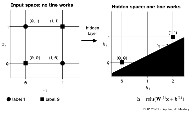
The hidden layer moves the points. In the input space (left) the classes sit on crossed diagonals. In the hidden space (right) the two points labelled 1 land on the same spot, and a single straight line separates the classes.
The hidden layer sends \({(0, 1)}\) and \({(1, 0)}\) to the same point, \({(1, 0)}\). The two points labelled 0 go to \({(0, 0)}\) and \({(2, 1)}\), one on each side of it. Three points in a row with the odd one in the middle would still be hopeless, but these three are not in a row: the middle one sits below the line through the other two. So a line can cut it off.
That is the whole trick of a multilayer perceptron. The hidden layer is a learned change of coordinates. The output neuron is still a plain linear model, as in DL01.1, but it works on the new coordinates, where the problem has become linear. In DL01.1.4 we fixed XOR by hand with the feature \({x_1 x_2}\). Here the network computes its own features.
Build it up
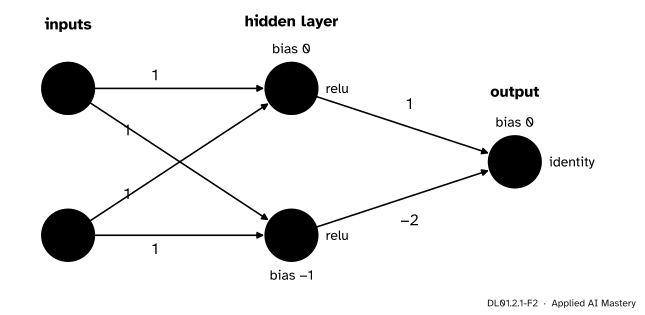
Step 1. The network. Two inputs, two hidden units, one output: a 2-2-1 network. Each hidden unit is a neuron from DL01.1 with the ReLU activation, \({\mathrm{relu}(z) = \max(0, z)}\). The output neuron has no activation at all: it is the identity, and we predict label 1 when its output is above 0.5. These are the weights of Goodfellow et al., section 6.1.
DL01.2.1-F2
The hand-built XOR network. Every weight and bias sits on the part it belongs to.
Step 2. Both hidden units read the same sum. All four input weights are 1, so each hidden unit sees \({s = x_1 + x_2}\). The biases differ: \({h_1 = \mathrm{relu}(s)}\) and \({h_2 = \mathrm{relu}(s - 1)}\). The first unit switches on as soon as \({s > 0}\); the second waits until \({s > 1}\).
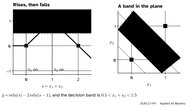
Step 3. The output subtracts twice the late unit. With output weights 1 and \(-2\) and no bias, \({\hat y = h_1 - 2h_2}\). While only \(h_1\) is on, the output climbs with \(s\). Once \(h_2\) joins in, it subtracts twice as fast as \(h_1\) adds, so the output turns round and falls.
Step 4. Read the picture. The output rises then falls as \(s\) grows, so it is large only for middling \(s\). The XOR points have \({s = 0, 1, 1, 2}\): the label-1 points are exactly the middling ones.
The formal statement
A network with one hidden layer of \(n_1\) units maps an input \(\vect{x}\) in \(\R^d\) to an output in two steps. Following the course notation, the hidden layer computes
Call \({s = x_1 + x_2}\). Then \({h_1 = \mathrm{relu}(s)}\), \({h_2 = \mathrm{relu}(s - 1)}\) and \({\hat y = h_1 - 2h_2}\). Take the three ranges of \(s\) one at a time.
If \({s \le 0}\), both units are off: \({\hat y = 0 - 0 = 0}\).
If \({0 \le s \le 1}\), only \(h_1\) is on: \({\hat y = s - 0 = s}\).
If \({s \ge 1}\), both are on: \({\hat y = s - 2(s - 1) = 2 - s}\).
The pieces agree where they meet (at \({s = 0}\) both give 0, at \({s = 1}\) both give 1), so the output is a continuous tent in \(s\): up with slope 1, then down with slope \(-1\).
DL01.2.1-F4
The output depends on the input only through \({s = x_1 + x_2}\). It is above 0.5 for \({0.5 < s < 1.5}\), which in the plane is a band between two parallel lines. A single neuron can only draw one line; the hidden layer lets the network draw two.
So the network predicts 1 exactly when \({0.5 < x_1 + x_2 < 1.5}\). In the input space that region is a band, not a half-plane, and no single neuron can produce a band. In the hidden space the same rule is the half-plane \({h_1 - 2h_2 > 0.5}\), which is the output neuron’s own decision rule.
Go deeper: why the nonlinearity is essential
Remove the ReLU and the hidden layer becomes affine: \({\vect{h} = \mat{W}^{(1)}\vect{x} + \vect{b}^{(1)}}\). The output is then
one affine function of \(\vect{x}\), which DL01.1.4 showed cannot separate XOR. Exercise 3 proves it directly. The ReLU breaks the chain because it is not affine: it bends at zero.
Worked example
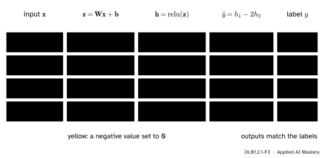
Push all four inputs through the network, one column at a time.
DL01.2.1-F3
The trace of the hand-built network. The ReLU acts only once, on the first row, where it turns \(-1\) into 0. The outputs equal the labels.
Input \({(0, 0)}\).\({\vect{z} = (0 + 0 + 0,\; 0 + 0 - 1) = (0, -1)}\). The ReLU keeps 0 and turns \(-1\) into 0, so \({\vect{h} = (0, 0)}\) and \({\hat y = 0 - 2 \cdot 0 = 0}\).
Input \({(0, 1)}\).\({\vect{z} = (1, 0)}\), nothing negative, so \({\vect{h} = (1, 0)}\) and \({\hat y = 1 - 0 = 1}\).
Input \({(1, 0)}\). The same sum, so the same values: \({\vect{h} = (1, 0)}\) and \({\hat y = 1}\).
Input \({(1, 1)}\).\({\vect{z} = (2, 1)}\), so \({\vect{h} = (2, 1)}\) and \({\hat y = 2 - 2 \cdot 1 = 0}\).
Every output equals its label, so with the threshold 0.5 all four predictions are right, with no margin of doubt: the outputs are exactly 0 or 1.
The line in hidden space. The output neuron predicts 1 when \({h_1 - 2h_2 > 0.5}\). Check the three hidden points: \({(0, 0)}\) gives 0, \({(1, 0)}\) gives 1, \({(2, 1)}\) gives 0. Only the label-1 point is above 0.5. Any threshold strictly between 0 and 1 would do; 0.5 sits in the middle.
Code
First the hand-built network, from scratch, with the examples as rows of a matrix.
import numpy as npX = np.array([[0, 0], [0, 1], [1, 0], [1, 1]], dtype=float)y = np.array([0, 1, 1, 0])def relu(z):return np.maximum(z, 0.0)W1 = np.array([[1.0, 1.0], [1.0, 1.0]]) # shape (out, in), as in the courseb1 = np.array([0.0, -1.0])W2 = np.array([1.0, -2.0])b2 =0.0Z1 = X @ W1.T + b1 # one row per exampleH = relu(Z1)y_hat = H @ W2 + b2print("hidden values:", H.tolist())print("outputs: ", y_hat.tolist())print("predictions: ", (y_hat >0.5).astype(int).tolist())
Now the network of M05.9: two tanh hidden units, a sigmoid output and the mean log loss, from the starting weights fixed in M05.9.1, trained for 300 full-batch steps with learning rate 1, exactly as in M05.9.2.
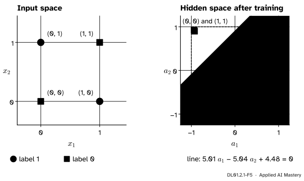
The learned features are not the hand-built ones. This network sends the two label-0 points, \({(0, 0)}\) and \({(1, 1)}\), to nearly the same corner, about \({(-0.93, 0.91)}\), and pushes the label-1 points to opposite corners. The line \({5.01\,a_1 - 5.04\,a_2 + 4.48 = 0}\) then separates them.
DL01.2.1-F5
The trained tanh network solves XOR the other way round: it merges the two label-0 points and keeps the label-1 points apart. Different features, same job. The weights are rounded; a different machine may change the last digit.
Finally, a library check that the hidden space is what makes the problem linear. scikit-learn’s Perceptron (the learning rule of DL01.1.2) can only draw one line.
from sklearn.linear_model import Perceptrondef perceptron_accuracy(features): model = Perceptron(max_iter=1000, tol=None, random_state=0).fit(features, y)return model.score(features, y)print("on the inputs: ", perceptron_accuracy(X))print("on the ReLU features: ", perceptron_accuracy(H))print("on the learned features:", perceptron_accuracy(A1))
on the inputs:           0.5
on the ReLU features:    1.0
on the learned features: 1.0
On the raw inputs the perceptron never settles (here it ends with two of the four points right), and no line can get more than three. On either set of hidden features it gets all four.
Explore
The module’s interactive, hinges and folds, lives in lesson DL01.2.4. It builds on the idea of this lesson: ReLU units bend a straight line, and enough bends make any shape.
Pitfalls
DL01.2.1-F6
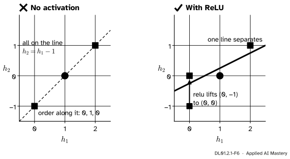
Wrong beside right. Without an activation the hidden points stay on one line, in the order 0, 1, 0, and no line can pick out the middle one. The ReLU lifts \({(0, -1)}\) to \({(0, 0)}\), off that line.
“More layers always add power, activation or not.”
Layers without an activation compose into one affine map, so a stack of them is no stronger than a single neuron (the deeper block above). The figure shows it in hidden space: the affine features \({(0, -1), (1, 0), (1, 0), (2, 1)}\) all lie on the line \({h_2 = h_1 - 1}\), labelled 0, 1, 1, 0 in order, and no line can separate the middle of a row from its two ends.
“The network learns the clean solution from the textbook.”
Gradient descent finds some solution, not a particular one. The trained tanh network merged the label-0 points instead of the label-1 points. Goodfellow et al. make the same point about this example: gradient descent would usually not find the clean integer weights. Read hidden units by what they do to the data, not by hoping for a familiar formula.
“A hidden unit that outputs zero is broken.”
For the input \({(0, 0)}\) both hidden units output 0, and the network is still right. A ReLU unit that is off for some inputs is doing its job: being off is how it bends the function. A unit that is off for every input is a different matter, the dead units of DL01.3.2.
Check yourself
Recall
1. Where does the hidden layer of the hand-built network send the input \({(0, 1)}\), and where does it send \({(1, 0)}\)?
Show answer
Both go to \({(1, 0)}\): each has \({x_1 + x_2 = 1}\), so \({h_1 = \mathrm{relu}(1) = 1}\) and \({h_2 = \mathrm{relu}(0) = 0}\).
2. Write the output of the hand-built network as a function of \({s = x_1 + x_2}\) on the three ranges of \(s\).
Show answer
0 for \({s \le 0}\), \(s\) for \({0 \le s \le 1}\), and \({2 - s}\) for \({s \ge 1}\): a tent with its peak 1 at \({s = 1}\).
3. Which line separates the classes in the hidden space of the hand-built network?
Show answer
\({h_1 - 2h_2 = 0.5}\). The label-1 point \({(1, 0)}\) gives 1, above 0.5; the label-0 points \({(0, 0)}\) and \({(2, 1)}\) give 0.
4. Why can a stack of layers without activations not solve XOR?
Show answer
Affine maps compose into one affine map, so the whole stack is a single neuron’s linear score, and no line separates XOR.
5. How do the hidden features of the trained tanh network differ from the hand-built ones?
Show answer
It sends the two label-0 points to nearly the same corner, about \({(-0.93, 0.91)}\), and the label-1 points to opposite corners; the hand-built network merges the label-1 points instead.
Exercises
1.★ Feed the point \({(0.5, 0.5)}\) and the point \({(1, 0.8)}\) to the hand-built network. Give the hidden values, the outputs and the predicted labels.
Show solution
For \({(0.5, 0.5)}\), \({s = 1}\), so \({\vect{h} = (\mathrm{relu}(1), \mathrm{relu}(0)) = (1, 0)}\) and \({\hat y = 1}\): label 1. For \({(1, 0.8)}\), \({s = 1.8}\), so \({\vect{h} = (1.8, 0.8)}\) and \({\hat y = 1.8 - 1.6 = 0.2}\): below 0.5, label 0. Both agree with the band \({0.5 < s < 1.5}\).
2.★★ A different network uses \({h_1 = \mathrm{relu}(x_1 - x_2)}\), \({h_2 = \mathrm{relu}(x_2 - x_1)}\) and \({\hat y = h_1 + h_2}\). Give its weights and biases, compute the hidden values of the four XOR points, and show that it solves XOR. What function of \(\vect{x}\) is \(\hat y\)?
Show solution
The first layer has rows \({(1, -1)}\) and \({(-1, 1)}\) and zero biases; the output weights are \({(1, 1)}\) with zero bias. The hidden values are \({(0, 0)}\) for \({(0, 0)}\), \({(0, 1)}\) for \({(0, 1)}\), \({(1, 0)}\) for \({(1, 0)}\) and \({(0, 0)}\) for \({(1, 1)}\). So both label-0 points land on the origin, and the outputs are 0, 1, 1, 0: correct. In hidden space the line \({h_1 + h_2 = 0.5}\) separates them. Since \({\mathrm{relu}(u) + \mathrm{relu}(-u) = \abs{u}}\), the output is \({\hat y = \abs{x_1 - x_2}}\). Like the tanh network, this one merges the label-0 points.
3.★★★ Take a 2-2-1 network whose hidden layer has no activation, as in the deeper block. Prove that it cannot output more than 0.5 on \({(0, 1)}\) and \({(1, 0)}\) and less than 0.5 on \({(0, 0)}\) and \({(1, 1)}\), whatever its weights.
Show solution
Multiply out, as in the deeper block: \({\hat y = \vect{w}\T\vect{x} + c}\) with \({\vect{w}\T = \mat{W}^{(2)}\mat{W}^{(1)}}\) and \({c = \mat{W}^{(2)}\vect{b}^{(1)} + b^{(2)}}\). Write \(f\) for this function and add its values in pairs:
Both sums equal \({w_1 + w_2 + 2c}\). The wanted inequalities make the first sum less than \({0.5 + 0.5 = 1}\) and the second greater than 1, so they cannot be equal. No weights work.
Summary card
A hidden layer changes the coordinates until the problem is linear.
DL01.2.1-F1
Crossed diagonals become separable.
Hidden layer.\({\vect{h} = \phi(\mat{W}^{(1)}\vect{x} + \vect{b}^{(1)})}\), then a linear output \({\hat y = \mat{W}^{(2)}\vect{h} + b^{(2)}}\).
The XOR network.\({h_1 = \mathrm{relu}(s)}\), \({h_2 = \mathrm{relu}(s - 1)}\), \({\hat y = h_1 - 2h_2}\) with \({s = x_1 + x_2}\).
Its decision rule. A band, \({0.5 < x_1 + x_2 < 1.5}\), which one neuron cannot draw.
The activation is essential. Without it the layers collapse into one affine map.
Sources and next steps
Sources. Each was opened and checked against this lesson on 15 November 2026.
Ian Goodfellow, Yoshua Bengio and Aaron Courville, Deep Learning, chapter 6, MIT Press. Section 6.1, Learning XOR, gives the hidden weights, biases and output weights used here, the hidden values of the four points after the rectified linear step (equation 6.10) and the outputs 0, 1, 1, 0 (equation 6.11), with the remark that gradient descent would usually not find such clean integer solutions.
Simon J. D. Prince, Understanding Deep Learning, MIT Press, free PDF. Sections 3.1 and 3.2 build a shallow network from ReLU hidden units and show each hidden unit adding a joint to a piecewise linear function, the view this module develops.
Aston Zhang, Zachary Lipton, Mu Li and Alexander Smola, Dive into Deep Learning, section 5.1. Hidden layers, the batch equations with examples as rows, and the argument that an affine function of an affine function is affine, so a hidden layer needs a nonlinear activation.